Un-confusing the Confidence Interval

A crucial acknowledgement of the scientific method is that no measurement will ever be perfect: results will always have associated variability, no matter how sophisticated the methodology used. Bioassay is no exception, so it is not surprising that one of the most common areas we address at Quantics is how to account for this uncertainty. When estimating a quantity, for example the EC₅₀ of a new test lot, we can account for uncertainty by using a confidence interval (CI).  Over this 3-part series of blogs, we’re going to demystify the confidence interval, and help give you an understanding of what a CI means – and how they are calculated – which you can take into your next bioassay.

In this first part, we’re going to lay the groundwork by discussing the basic ideas of variability within the context of bioassay, which is essential for understanding and interpreting the confidence interval.

One common problem in which we might be interested in a bioassay context is to estimate the EC₅₀ of a test lot: the dose at which half the maximum response is observed. Every test lot will have a “true” EC₅₀ – this is the value we want to know.

In a sense, however, we can never actually access this “true” value due to the variability of any experiment we perform to measure the EC₅₀. Instead, we use the values we measure in these experiments to help us infer a probable value for the “true” EC₅₀.

In statistics, we generally refer to  the “true” value as a parameter and sample-based estimates as statistics. Parameters are statistical properties of an entire population, such as a politician’s approval rating. Statistics are properties of a subset of that population, such as the results of opinion polls of a (hopefully) representative sample of voters.

Statistics are used to estimate parameters: we recognise that no one poll gives the “true” approval rating for the entire population, but we can use several polls to form an estimate.

So, we know that we can’t actually measure the “true” value of our sample’s EC₅₀ directly, only infer it from our sample data. But what does this look like in practice?

A helpful way to think about the problem is to look at the distribution of the (sample) EC₅₀values. This defines the range of possible values for the EC₅₀, as well as how likely those values are to be observed when a sample is taken. One common distribution in statistics is the normal distribution, which many of you would recognise as a classic “bell-curve”. We’re going to consider only normally distributed values here – in part 2, we’ll expand this further.

One note here: strictly speaking, it is the log(EC₅₀) which is typically observed to follow a normal distribution. In this blog, we’re going to assume that all EC₅₀s are measured on the log scale for the sake of simplicity (and to avoid writing “log” a million times!).

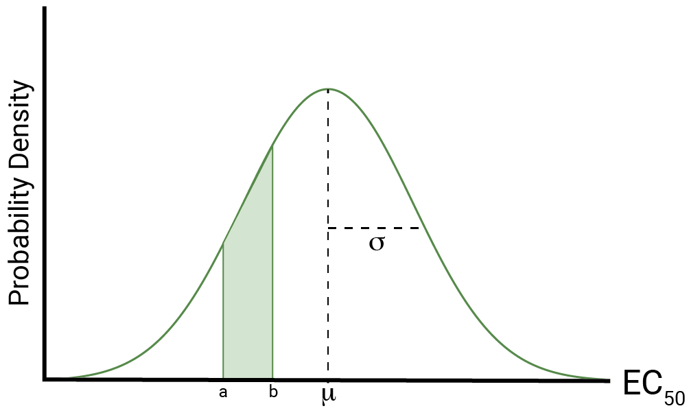
We can uniquely define the normal distribution of our EC₅₀ estimates by two parameters – the mean and the standard deviation, which we denote as µ and σ respectively. Figure 1 shows an example. The mean is the central value around which the bulk of the probability is distributed which, assuming the assay is unbiased, will be the “true” EC₅₀ of the test lot.

The standard deviation, conversely, tells us about how variable the measurement of the EC₅₀ is. It represents a ‘typical’ deviation between an observation and the mean. If the standard deviation is large, then the distribution will be wider.

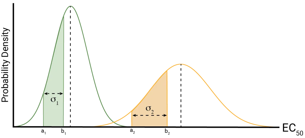
Whenever we make a measurement of our EC₅₀, we are effectively drawing a value from its distribution. For the normal distribution, the probability of observing a value within a particular interval is represented by the area under the curve. This means we are more likely to observe values near the peak of the curve, and less likely to observe those near the tails of the distribution. As the standard deviation increases, the distribution will get wider; as such, it is more likely to observe a value further away from the mean (in absolute terms) than for a narrower distribution. This is shown in Figure 2.

The ultimate goal of our assay is to estimate the mean of the distribution – the “true” EC₅₀ – as well as its standard deviation. The latter is vital, since we need to understand the uncertainty of our measurements. The problem is that these are parameters: we cannot directly measure them since they are properties of the population.

We can, however, use statistics based on repeated measurements of the EC₅₀ (or a sample) to estimate these parameters. Our sample will itself have a mean and standard deviation – these are the statistics we use to estimate the parameters of the distribution.

We use different notation to differentiate these from the mean and standard deviation of the  population. If we denote the measurements of the EC₅₀ by, say, , then the mean is referred to as , and the standard deviation is given by .

This is probably best illustrated using a concrete example. Let’s imagine the “true” EC₅₀ of our test lot is 3, and the standard deviation of its distribution is 0.5. In the real world, however, we would not know the “true” EC₅₀ and its standard deviation in advance.  Suppose we then collect a dataset with  a sample of 10 measurements of the EC₅₀.

Using a bit of high school maths (or Excel), we can work out that, for this set of data:

So, the sample mean is slightly lower than the population mean (“true” EC₅₀). Conversely, the sample standard deviation is slightly higher than that of the population.

From just these two numbers (the sample mean and the sample standard deviation), we have no idea whether we’ve got the answer right, or how far out we are likely to be. The good news is that, with a little bit more work, we can construct a confidence interval to get a very good sense of where our true EC₅₀ is likely to lie. That’s going to be the subject of part 2 of this series, so be sure to sign up to our blog mailing list so you don’t miss a thing!

Need a stats refresher? Check out out Stats 101 training course here: https://www.quantics.co.uk/biostatistics-services/basic-statistics-training/