Design of Experiments for Bioassay Optimisation (with RoukenBio)

So, you’re confident that you’ve got a feasible assay with a well-defined dose-response curve. But bioassays, as we all know, are fickle. The observed responses are sensitive to many factors which can lead to appreciable variability in the experiment and, in turn, a high assay failure rate. An important part of the development phase of an assay, therefore, is to efficiently determine the preparation and environment which allows for the greatest chance of a high-performing assay. This can be achieved using Design of Experiments or DoE.

This blog post is a collaborative effort between RoukenBio’s stellar bioanalytical team and Quantics, showcasing a real-world case study of how Design of Experiments (DoE) is applied to bioassay data. Together, we’ve worked to highlight the practical value and insights that can be gained through DoE methodologies in optimising bioanalytical processes. For those interested in exploring more about the foundational aspects of bioassays, check out our first collaborative blog: Potency Assays: The Cornerstone of Biotherapeutic Development.

DoE is not a process unique to bioassays, or even to biology. It is a statistical technique used in a wide range of fields and contexts to analyse how experimental conditions – or factors – influence the outcome of the experiment. Specifically, the advantage of a DoE approach is to allow several factors to be varied at the same time while still giving information about the influence of each factor individually.

For a toy example, imagine a gardener is growing a prize lettuce, and wants optimal growing conditions so it turns out as big as possible. She needs to find out how much she needs to water the lettuce, and what percentage of each day she needs to turn on the lights in her indoor greenhouse.

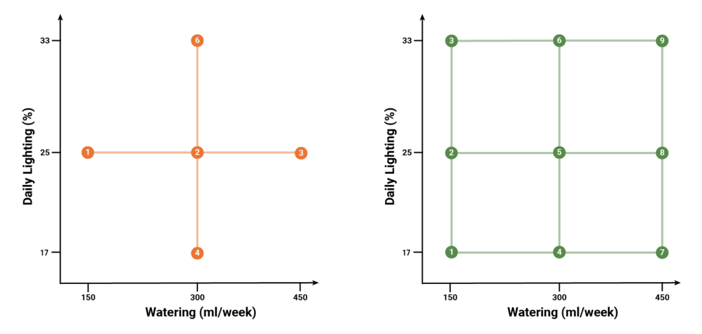
Traditionally, she might grow three trial plants with different levels of watering and the same level of light. In parallel, she might then grow three plants with differing levels of lighting and the same amount of water. She might determine the levels of water and light which grew the largest lettuce, and use those levels to grow the prize lettuce. This approach – holding one factor constant while varying the other – is known as a One Factor At a Time (OFAT) design. The table below shows an example of a OFAT experiment for finding a lettuce’s optimal growing conditions.

One key downside of this method, however, is that it can be very difficult to determine if there are any interactions between the two factors. What if, for example, the optimal conditions would be to maximise both watering and lighting in the range tested? We might intuit this from the results of the OFAT experiment, but we have no experimental evidence for this conclusion as this was not a combination which was tested.

How else could our gardener approach the problem? This is where we enter the realm of design of experiments. Our goal is to maximise the information gained in our trial while keeping the number of experimental runs as small as possible. We are looking to make our information gathering procedure as efficient as possible. There are a wide range of different designs, some of which we will encounter later, but perhaps the easiest to understand is the full factorial design. Simply put, we test every combination of factors and see which performed best. While this can result in many runs, it provides the most possible information about the behaviour of the experiment.

If the gardener used a full factorial design, her trials might look like this:

Figure 1 displays the two approaches as networks in design space: the left diagram shows the network for an OFAT experiment, while the right diagram shows the network for a full factorial designed experiment. In both, the nodes are labelled with the run number they represent. It is clear that far more of design space is covered in the full factorial experiment than in the OFAT experiment for the addition of only three extra runs. This means our gardener is more likely to find the best growing conditions for her lettuce.

Further, performing runs on the “corners” in design space now means we can better understand how the two factors interact with each other. That is, these are combinations of the factors which were not tested in an OFAT experiment which could allow us to spot any synergistic effects.

Just as a prize lettuce requires the optimal growing conditions to win at the town fair, it is important to consider the conditions and procedure of performing a bioassay to help ensure optimal performance. As you might expect, therefore, DoE provides an excellent tool for deciding the best assay design.

Bioassay has been slower to adopt a DoE approach to assay design compared to some other fields in the life sciences. Some of the hesitancy to employ DoE is simply down to lack of awareness of the technique, but it is also perceived as a complicated and difficult approach which requires significant resources to implement. This doesn’t need to be the case: a well-thought-out DoE procedure can provide significant benefits in performance over the lifetime of an assay for comparatively minor up-front cost.

We’re going to walk through the DoE process for a real bioassay, both to illustrate how the ideas of DoE can be applied in a bioassay context and to demonstrate the real savings that can be found. This will use real-world bioassay data collected in the lab by our colleagues at RoukenBio with their extensive experience of designing and implementing complex assays.

As is always the case in bioassay, the goal is to develop an assay which is accurate, precise, and robust. A successful DoE process for a bioassay, therefore, will determine the assay conditions and procedure which best supports its overall performance.

To optimise our assay, we’ll examine the asymptote difference: the difference between the upper and lower asymptotes of the 4PL curve used to model the assay data. This is a measure of the signal strength relative to the background noise in the assay. A potency assay with a large asymptote difference is more robust, as it produces a clear, easily detectable signal while minimising interference from background noise. This improves assay precision and ensures that variations from unintended factors—such as temperature fluctuations on a hot summer’s day—have a proportionally smaller impact on the results. A strong signal also enhances the reliability of potency calculations, reducing variability and making the assay more resilient to operational changes.

The asymptote difference is a commonly used parameter in a bioassay DoE, but other assay properties can be used to further inform the process. These might include the assay’s hill slope or EC₅₀, for example.

So, what factors do we need to consider for our bioassay DoE? RoukenBio were developing an interleukin-13 (IL-13) neutralisation assay, where a baseline assay response is achieved using cells engineered to express luciferase in response to IL-13. A neutralising test article is introduced in a dose dilution series to sequester IL-13 and block the downstream signalling that results in luminescence. Three main influencing factors were selected to be focused on:

• Cell Density (cells/well): The number of cells included in each well on the plate. In general, a stronger response can be expected by seeding more cells. However, too many cells can result in overcrowding, ultimately leading to cell death and a weakened response. This means a cell number which balances response strength and cell health must be found.
• Cytokine Stimulation (ng/ml): Cytokines are a type of small protein which form a crucial part of the immune system. In this assay, IL-13 is required to stimulate a baseline response (the maximal signal response). It is important, therefore, to determine an optimal concentration of cytokine to be added in the assay.
• Incubation time (hrs): Bioassays are typically left in an incubator for a period of time after they are plated to allow the critical interactions to take place. The length of time for which an assay plate is incubated is crucial for ensuring optimal assay performance. Practical considerations, such as lab opening hours, are typically also typically taken into account alongside pure performance.

We chose to examine these factors at three indicative levels each.

As in our lettuce example, we chose a full factorial design. This tests every possible combination of factors and levels, meaning that, for three factors at three levels each, we require 27 assay conditions for the full experiment. This case allowed for a full factorial design as we had a small number of factors and levels to be tested. If more factors or levels are required, however, the number of conditions for a full factorial design can quickly escalate. A full factorial design with four levels of four factors would require 256 conditions, for example, so a different design requiring fewer data points might be chosen.

For assay runs in a DoE process, it is recommended that each run is performed on a single plate, by the same analyst, and over as short a time as is feasible. The intention here is to understand the effect of the factors of interest with as little influence from other sources of variability as possible. However, multiple conditions can be assessed within each plate and each run, allowing for several conditions to be evaluated in parallel.

In our case, assays were run in the RoukenBio lab for each combination of the three levels of the factors according to the full factorial experimental design. Three high throughput, 384-well plates were prepared, one per incubation time point, and each condition was measured in triplicate over each assay plate. Once the plates were analysed, a statistical model was fit to the data – the data in this case fit a 4PL model. These model fits are then used to evaluate our properties of interest in the DoE. The results from one run were unable to be fit using a 4PL model due to a very shallow response. The full results are shown in the table below.

One way we could have analysed this data is to look at the relationship between the asymptote difference and each factor individually. To do this, we plotted the mean asymptote difference obtained for each run using a certain level of a factor against that level. This is shown in Figure 2.

These plots show that, as might have been expected, there is a positive correlation between the factors and the asymptote difference. There is, however, some degree of subtlety in this result. For one, the strength of dependence of the asymptote difference is not consistent across the three factors. Specifically, we observe a strong relationship with the cytokine stimulation and incubation time, but the dependence on cell density appears to be much weaker.

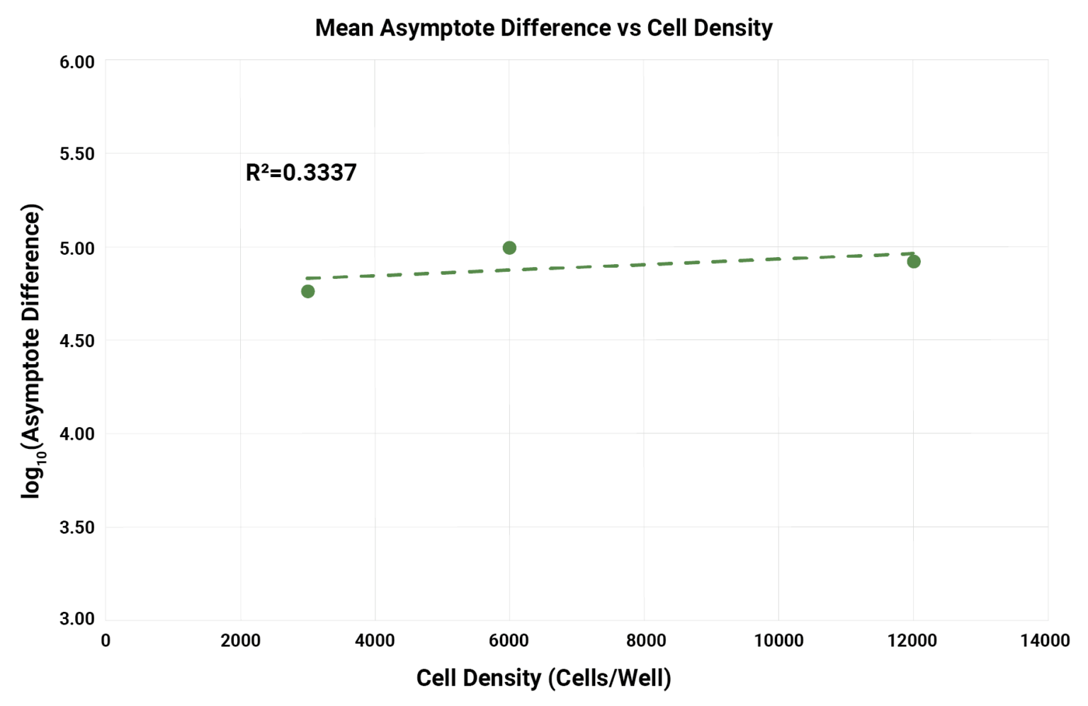
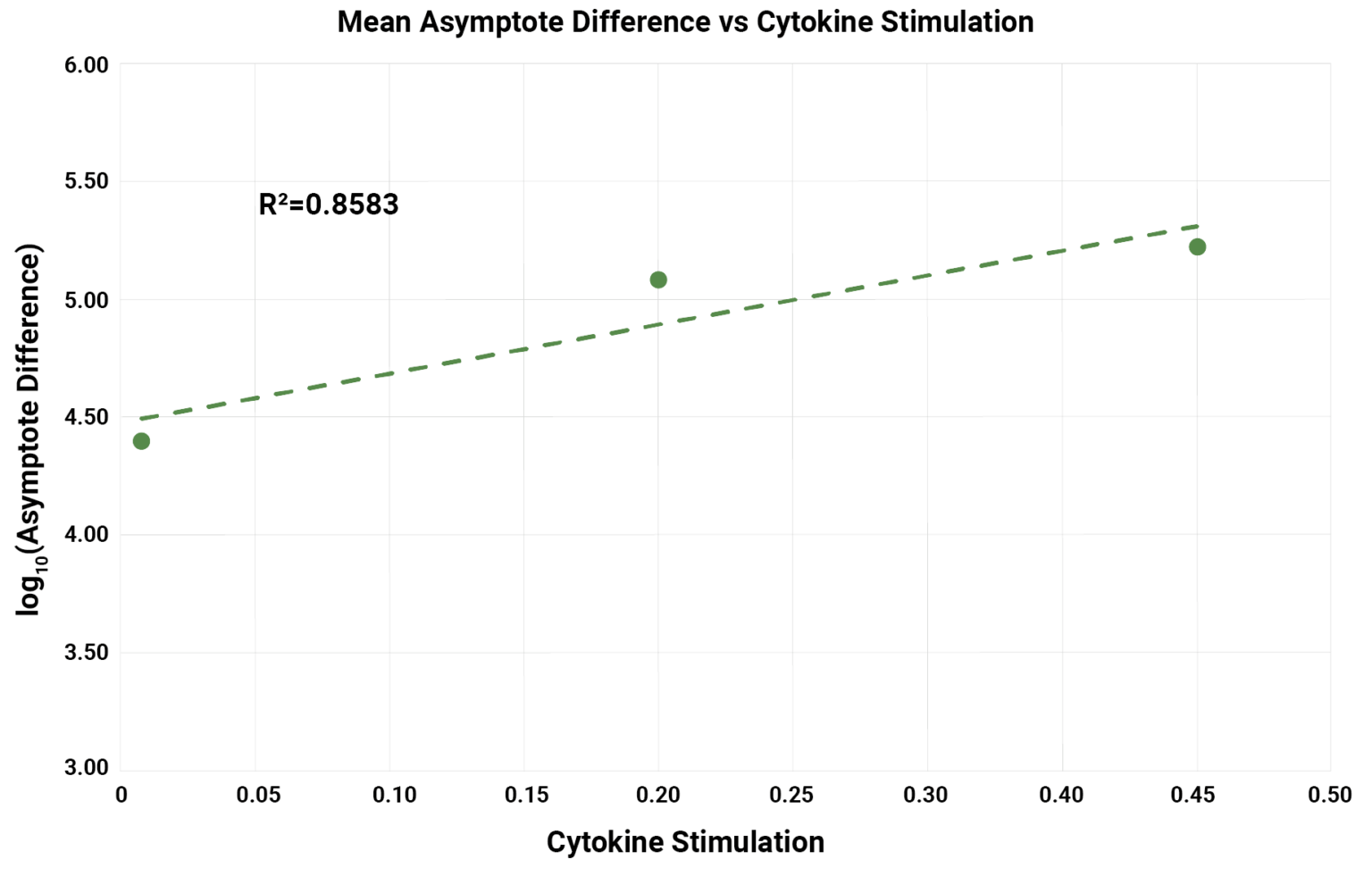
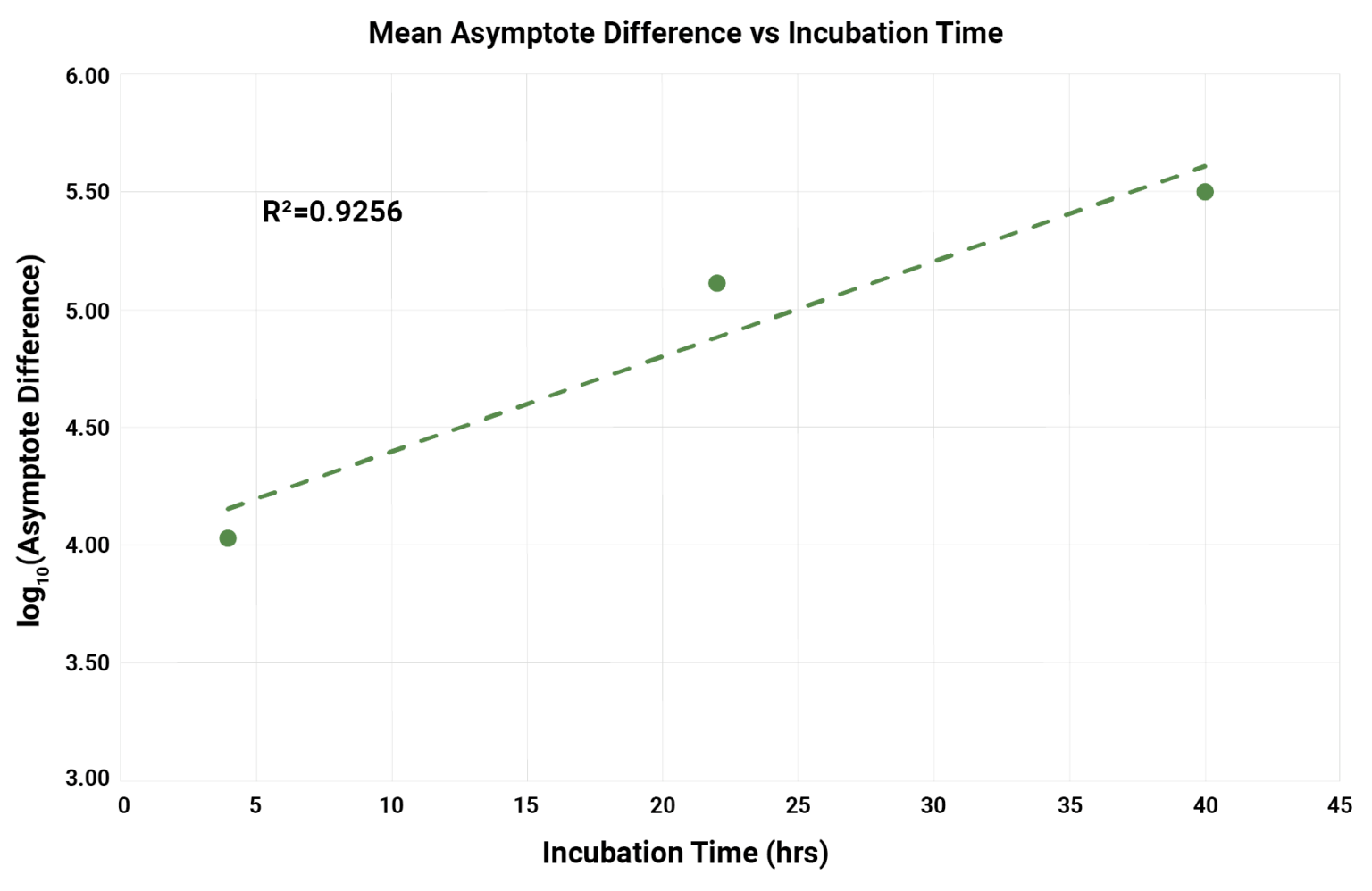
Most importantly, however, this process draws out the flaws of an OFAT approach. We would likely struggle to decide upon an optimal solution looking at each factor individually in this way. Asymptote difference shows a positive correlation with all three factors. We should maximise all three, right? But there’s also signs that we have non-linearity in the data – certainly the middle level for cell density gives a higher mean than the highest level! So maybe we should choose the middle levels?

As it happens, neither is actually the optimal combination of factors for our experiment! Using DoE – and, therefore, taking into account the interactions between the factors – we were able to find a better combination of experimental conditions for our assay.

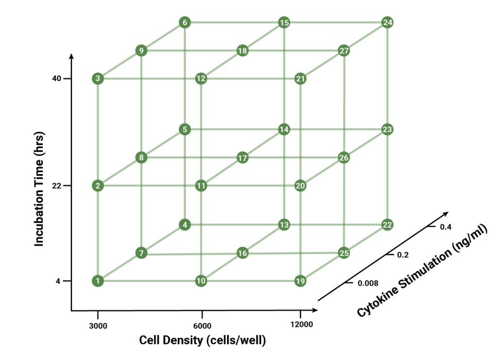
Figure 3 shows how the performed runs cover the design space for the experiment. Each point on the diagram is labelled by the number of the run it represents.

Since the results for asymptote difference were spread over several orders of magnitude, we have chosen to take a log transform of this data as our final result: essentially, we are just plotting the asymptote difference on a logarithmic scale.

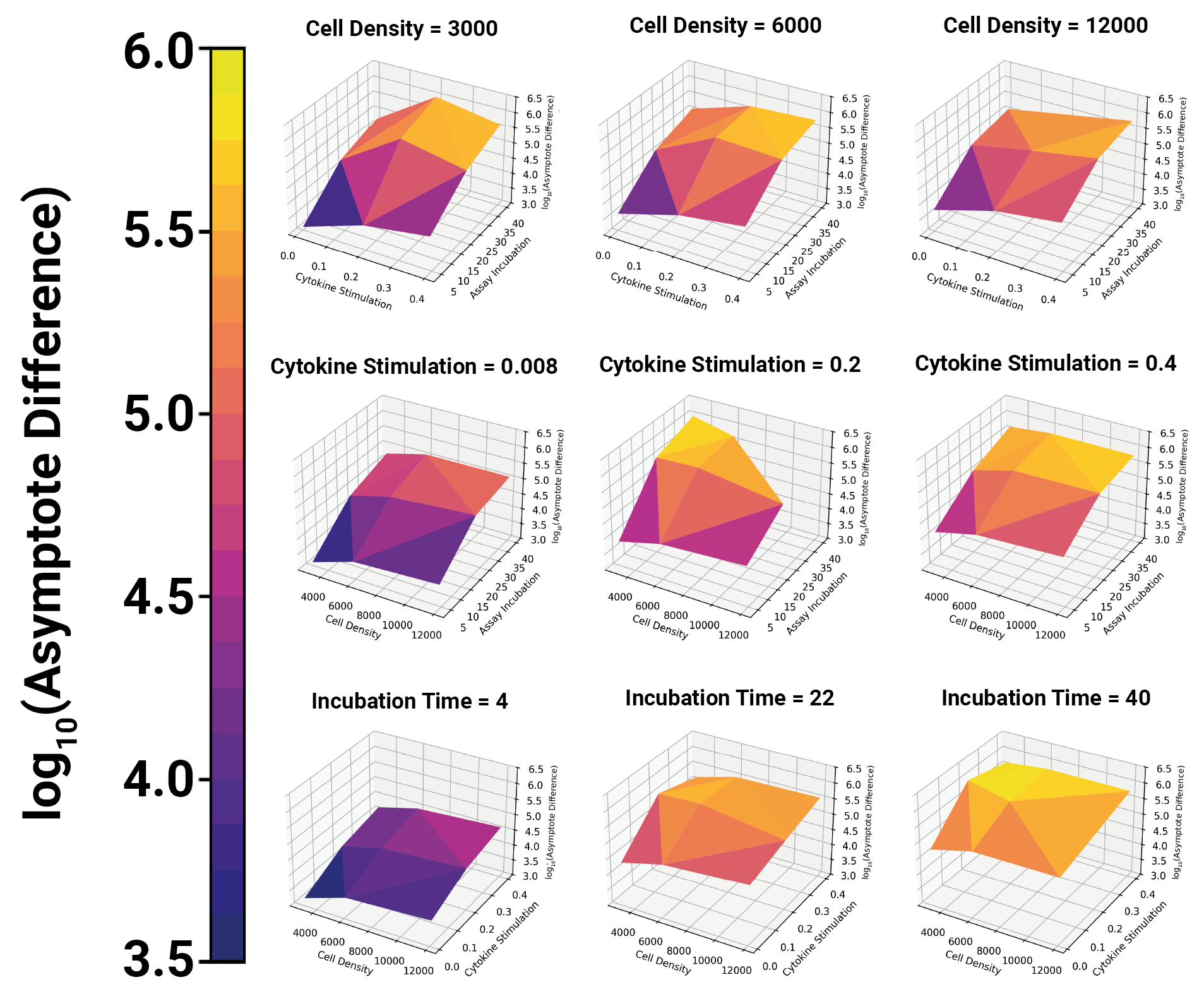
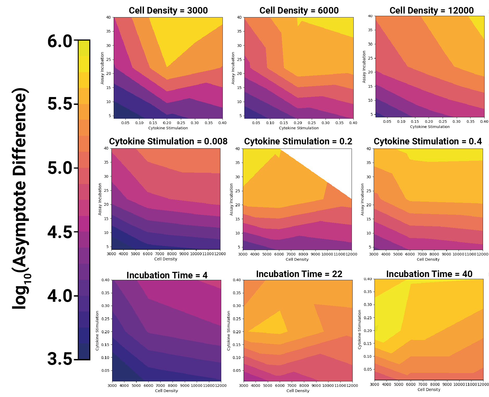
We represent the data as both 3D surface plots and with contour plots in Figure 4.

To produce these plots, each factor was held constant at each of its levels in turn. The asymptote difference is then plotted for each combination of the other factors and levels. For the 3D plot, this is shown on the z-axis and represented on the surface according to the colour bar.

These surfaces are mapped into two dimensions in the contour plots. The colour scheme is identical between the two types of plots: purples and blues indicate smaller asymptote differences, while oranges and yellows indicate larger asymptote differences. Since we are looking to maximise the assay range, combinations which result in yellow regions on the plots are desirable.

From the results, we can identify that the combination of factors which produces the maximum asymptote difference is:

Cell Density: 3000 cells/well

Cytokine Stimulation: 0.2 ng/ml

Incubation Time: 40 hrs

For this DoE process, we chose to use a full factorial design – testing every combination of the chosen levels – as this did not result in an unmanageable number of assay runs. It is, nevertheless, interesting to consider whether we could have determined the same optimal solution using a design with fewer runs.

We can use the results from our full factorial experiment to understand the results we might have obtained using a different design. The table below shows the results which would have resulted from a Box-Behnken design, which, in this case, requires only 13 runs compared to the 27 runs necessary for a full factorial experiment. The numbering of the runs has been maintained from the original results for consistency.

Figure 5 shows these runs in design space.

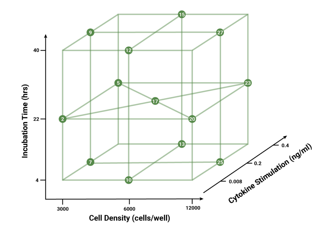
This design provides good coverage along all three axes while directly testing the midpoints of each factor, meaning we are likely to detect any curvature in the relationship between any of the factors and the asymptote difference. And indeed, in this case, we find that our optimal solution – run 9 – would have been obtained by this Box-Behnken design. This was, of course, no guarantee: if our optimal solution had been one of the corner runs – maximising all three factors, for example – then we would not have picked it up using this design. This demonstrates the trade-off between reducing the number of runs and the amount of information gained. Informed experimental designs such as Box-Behnken might maximise the amount of information gained from a reduced number of runs, but a full factorial design will always give you the best chance to find the optimal combination of levels for an assay.

As with many aspects of bioassay development, DoE is at its most powerful with both scientific and biological involvement. There will always be a balance required between minimising time and resource use and ensuring that the experimental design provides enough information that the optimal solution is likely to be found. A well-performed DoE process can result in significant precision and/or robustness gains for an assay, so it is often worth considering as a key component of assay development.