Non-parallelism and Biosimilars

Many of our readers will be familiar with our paper “Parallelism in Practice” (PDA Journal of Pharmaceutical Science and Technology, 2015) and how we examined the common methods used for evaluation of parallelism for bioassay. In this blog we’ll explain why the usual way of thinking about parallelism doesn’t always make sense when dealing with biosimilars; we’ll discuss why this is and some alternative ways of approaching parallelism.

The standard approach

First let’s briefly review the usual approach to parallelism. As we detail in this blog, the aim of a potency assay is to calculate the relative potency (RP) of a test sample compared to another sample, called the reference standard. The RP is assumed to be the same at all response levels.

Before calculating the RP, a parallelism test is always carried out. We go into detail on parallelism in this blog. There are various types of parallelism tests (which our paper details), but the aim of all of them is the same: to check whether the dose-response curves for the reference and test samples are parallel, i.e. that they differ only by a horizontal shift. If they are, this indicates the reference and test samples are “similar”, i.e the test sample behaves as a dilution of the reference standard. On the other hand if the curves are not parallel, the samples aren’t similar.

We would generally expect that parallelism tests will usually pass if the assay and samples are behaving normally. If the parallelism test passes, we continue to the next step: fitting a parallel model and calculating the RP.

If a parallelism test fails, this is generally taken as a sign that something is wrong (for example, the test sample may have degraded), and so usually no RP would be calculated if this happens.

Biosimilars

For some bioassays involving biosimilars, the situation may be different.

Biosimilars are copies of licensed biologic drugs (Reference Medicinal Products (RMPs)). A biosimilar manufacturer is likely to have a different manufacturing process (e.g. different cell line, raw materials, equipment, processes, process controls and acceptance criteria) from that of the RMP and no direct knowledge of the manufacturing process for the RMP.

Since biological products are complicated, these manufacturing process differences mean that a biosimilar is unlikely to be completely identical to the RMP. In order to be approved it must however be highly similar in both physiochemical and biological terms, with no clinically meaningful differences that could potentially impact the purity, safety or efficacy of the product. However, there are still likely to be minor differences which have been judged to be clinically insignificant.

Now let’s think about the impact of this on parallelism: in a bioassay in which the biosimilar is being compared to the RMP, there is no reason why the two substances should behave exactly as dilutions of each other – they are different materials after all. Therefore their dose-response curves may not be parallel.

Any lack of parallelism is interesting in itself and will feed into an assessment of biosimilarity, but it will also affect calculations of RP. If the non-parallelism is substantial, the assay will fail any reasonable parallelism test. This means that if we follow the usual approach, we would not be allowed to calculate the RP.

We might try to get around this problem by changing the parameters of the parallelism test to increase the pass rate. For example, for an equivalence test we could set very wide gateposts, or for an F-test we could set a very low critical p-value. We would then be “allowed” to fit a parallel model and calculate an RP. However, if we did this we would be using a parallel model that is a very poor fit to the data – and using a poorly-fitting model will always lead to unreliable conclusions. So any RP calculated like this would be meaningless. It would also beg the question of what the point of the parallelism test is if it is set up to pass very non-parallel data.

A better way to deal with this is to accept that the dose-response curves really are non-parallel, and to report measures of potency that take this into account. We’ll explain how this works by showing how we applied this idea to some real data.

Real data

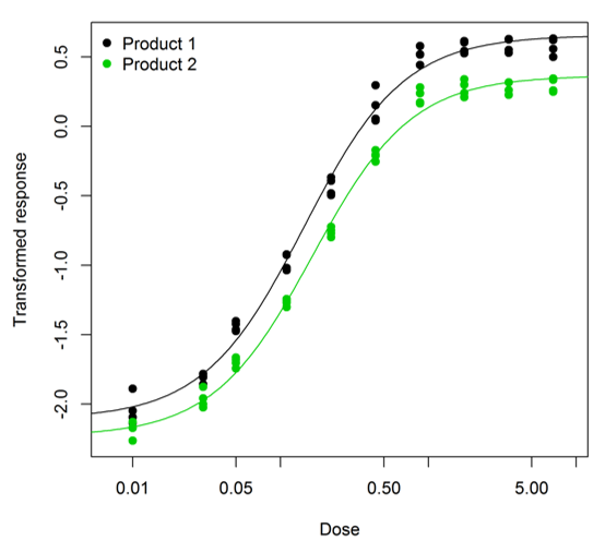
The assay we were looking at was an enzyme linked immunosorbent assay (ELISA) used as a surrogate for measurement of antibody-dependent cellular cytotoxicity (ADCC) activity, and included Product 1, the RMP, and Product 2, the biosimilar. The dose-response curve for both materials followed a four-parameter logistic. However, the curves were clearly non-parallel; the right asymptote for Product 1 was substantially higher than for Product 2. An example assay is shown below – you can clearly see that the curve for Product 2 (in green) levels off at a lower value than the curve for Product 1 (in black).

We saw the same pattern across all the assays we looked at (there were 20 in total). So fitting a parallel model clearly wouldn’t make sense. Instead we fitted a partly parallel model. What do I mean by “partly parallel”? This is easiest to explain by going back to the equation for the four-parameter logistic described in our earlier blog.

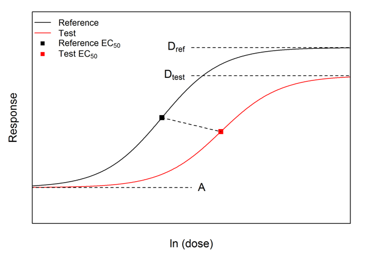
Here x = ln(dose), y is the response, and the parameters have the following interpretations: A and D are the left and right asymptotes (corresponding to zero and infinite doses respectively), C is the midpoint or ln(EC50), and B is the slope parameter.

For a parallel model, the above equation is used with separate C parameters for each curve, but common A, B and D parameters. For a non-parallel model, by contrast, all four parameters are separate for each curve. A partly parallel model is in between these extremes: some of the A, B and D parameters are forced to be equal for both the curves, but others are different for each curve.

After examining all 20 assays, we decided that the most suitable model was one in which the A and B parameters are the same for each curve, but the D parameters are not, allowing the right asymptotes to be different. We call this “Model AB”, since the A and B parameters are forced to be equal. Similarly, “Model A” would be one in which only the A parameters are equal, and so on.

For a parallel model, the above equation is used with separate C parameters for each curve, but common A, B and D parameters. For a non-parallel model, by contrast, all four parameters are separate for each curve. A partly parallel model is in between these extremes: some of the A, B and D parameters are forced to be equal for both the curves, but others are different for each curve.

After examining all 20 assays, we decided that the most suitable model was one in which the A and B parameters are the same for each curve, but the D parameters are not, allowing the right asymptotes to be different. We call this “Model AB”, since the A and B parameters are forced to be equal. Similarly, “Model A” would be one in which only the A parameters are equal, and so on.

Potency measures in Model AB

In model AB there are two differences between the dose-response curves: the C parameters differ, and the D parameters differ. Therefore the difference in potencies cannot be condensed into a single value. Instead, we used the following pair of values:

(1)  

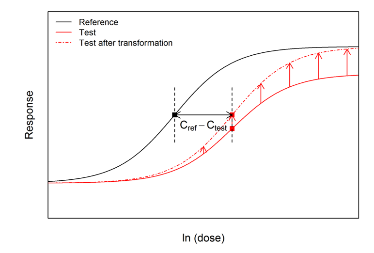
To aid the interpretation of this pair of numbers, the test curve can be ‘upscaled’ using a transformation of the responses determined by the ratio of ranges. The upscaled test curve can be shown mathematically to be parallel to the reference curve, and the horizontal distance between it and the reference curve is the difference between the original C parameters. Therefore the concept of RP can be applied correctly to the reference curve and the upscaled test curve. This ‘upscaling’ process is shown below:

Across the 20 assays, the average values we found for the two potency measures were 0.75 (with a 95% CI of 0.71 to 0.80) for the ratio of EC50s, and 0.911 (with a 95% CI of 0.908 to 0.914) for the ratio of ranges. If we’d ignored the lack of parallelism and fitted a parallel model anyway, the average RP we’d have found would have been 0.59 (with a 95% CI of 0.56 to 0.63) – substantially lower than the ratio of EC50s we actually found. So apart from the theoretical concerns, there is also a large practical impact.

Other models

For a different dataset, a different model might be appropriate. For example, if both the slope parameters and right asymptotes appeared to be consistently different, the best model would be “model A”. If a different model is used, the potency measures should be different as well. For model A, there are three differences between the curves: the B, C and D parameters are all different. So three potency measures should be used. In addition to the two potency measures from model AB, the ratio of B parameters should be reported as well.

Similarly for other models, other sets of potency measures would be appropriate. The number of potency measures reported should always be the same as the number of parameters which differ between the two curves.

Acknowledgements

This blog was developed from work we have done on the poster “Statistical approaches for reporting potency of Biosimilars” presented at BioPharmaceutical Emerging Best Practices Association Conference 2015 September.

Fleetwood K, Bursa F, Yellowlees A, Upsall A. Statistical approaches for reporting potency of Biosimilars. BioPharmaceutical Emerging Best Practices Association Conference Presented 2015 September.

Thanks are expressed to Drs. Daniel Galbraith, Terry Gray, Debbie Allan, Stefan Termén, Laura Munro and Lisa Blackwood (Technical Services, Sartorius Stedim BioOutsource) and Andy Upsall (Managing Director at Antibody Analytics)  for data collection, method expertise and technical discussion.