Response Transformation: When and How?
Our clients sometimes tell us that they don’t want to use response transformations since it feels like an unwarranted manipulation of the data. However, there is little point in avoiding a transformation just to get results that may be wrong. In this blog we explain when you should consider transforming the response, and how to choose a response transformation.
When analysing a relative potency assay, the dose itself is almost never used directly. Instead, a log transformation is applied, and the whole analysis is carried out using the log dose. This dose transformation is required for the relative potency calculation to make sense. (The only exception is for slope ratio assays, but these are rarely used.) In addition to transforming the dose, the response can also be transformed. Unlike the dose transformation, transforming the response is optional.
Key Takeaways
- Transforming responses helps meet the key statistical assumption of variance homogeneity, which is essential for reliable potency estimates.
- If variance increases with dose, square root or log transformations are often appropriate; if variance decreases, squaring or exponential transformations may work better.
- A constant coefficient of variation (CV) implies non-constant variance and typically indicates that a log response transformation is appropriate.
Testing variance homogeneity
First of all, response transformations should only be used for continuous data, never for quantal “all or none” data (e.g. alive or dead, or reacted / not reacted). In the rest of this blog we’ll only be talking about continuous data.
The underlying reason why a response transformation might be required is to satisfy the statistical assumptions made when fitting a dose-response model to the data. One of these assumptions is that the variance is “homogenous”. This means that the spread of the responses around the model is the same at every dose.
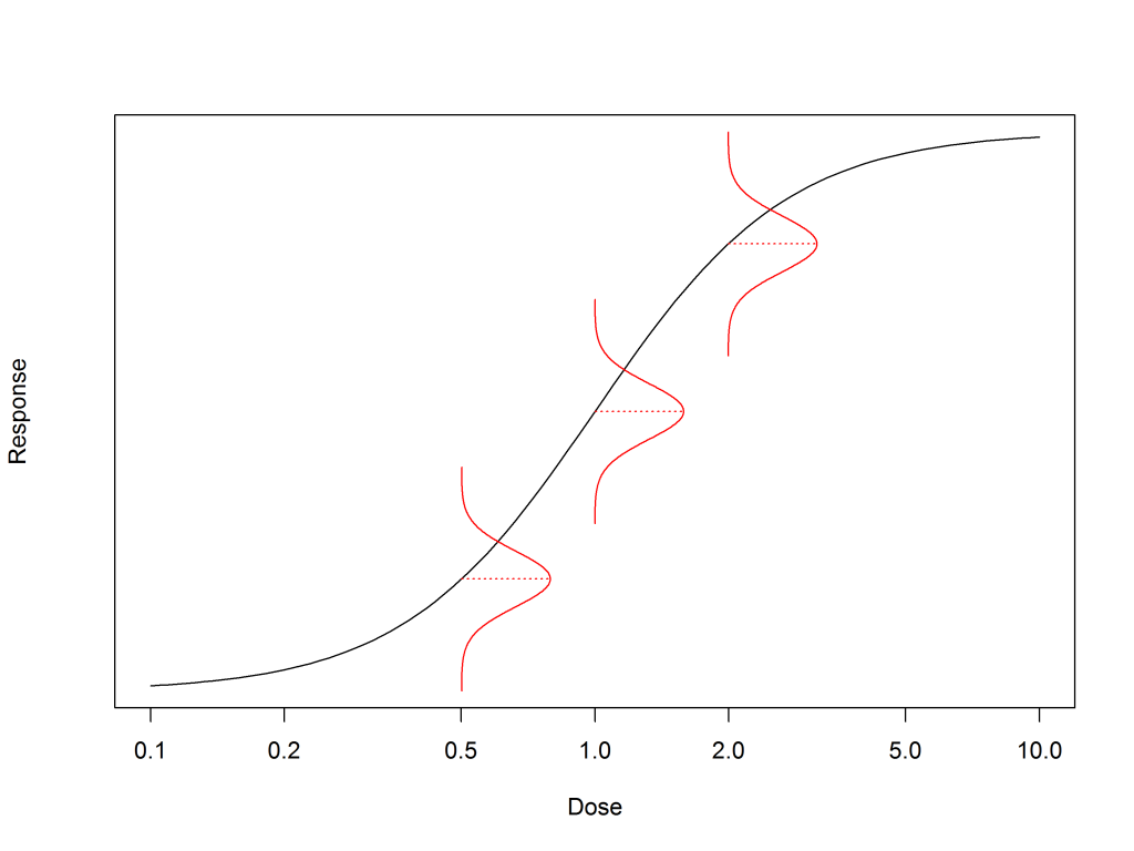
However, in practice this doesn’t always happen. An example is shown in Figure 2, where it is clear that the responses become more spread out at higher doses.
Sometimes the fact that the variability increases (or decreases) with the dose can be very obvious. In other cases it can be detected by calculating the standard deviation for each dose group. If the standard deviation is roughly the same for each dose group, the variance is homogenous; if not, this assumption is not valid.

Assessing variance homogeneity based on a single assay can be difficult, as each dose group may contain only a small number of replicates. Instead, multiple assays should be used. If they all show a consistent dependence of the standard deviation on the dose, it is likely that variance homogeneity is violated.
The coefficient of variation (often called the CV or %CV) of each dose group can also be used to test variance homogeneity. However, a constant CV means the standard deviation is not constant. This follows from the definition of the coefficient of variation:
\(CV = \frac{\text{Standard deviation of dose group}}{\text{Mean of dose group}}\)
Since the mean response varies with dose, the standard deviation must also vary in order to give a constant CV. Therefore, a constant CV is evidence that the variance is not homogenous.
Choosing a transformation
A lack of variance homogeneity can lead to serious problems. If the assumptions required for fitting are violated, the model fits will be inaccurate. This directly affects relative potency estimates, system and sample suitability criteria, confidence intervals and p-values.
The simplest way to address this is to transform the responses so that the variance becomes homogenous. In theory any transformation can be used, but a small number of simple transformations are very commonly effective and should usually be tried first.
If the standard deviation is higher for higher responses, common transformations include:
- \(\sqrt{\text{response}}\)
- \(\log(\text{response})\)
- \(\log(\text{response}+1)\), which is useful if the response can be zero
If the standard deviation is lower for higher responses, useful transformations include:
- \(\text{response}^2\)
- \(e^{\text{response}}\)
A particularly common situation is a constant CV. In this case it can be shown mathematically that a log(response) transformation should be used.
Transformations all the way down
Some people prefer to analyse “raw” data, feeling that response transformations represent an unwarranted manipulation. However, avoiding a transformation when assumptions are violated risks producing incorrect results.
In reality, most data has already been transformed. For example, optical density measurements are derived from light transmission using:
\(\text{Optical Density} = \log\left(\frac{\text{light input}}{\text{light transmitted}}\right)\)
This is itself a response transformation. In fact, even light transmission is derived from electrical signals produced by a photodiode, meaning multiple transformations occur before the data reaches us.
Truly “raw” data is rare, if it exists at all. Recognising this makes it easier to accept additional transformations when they improve statistical validity.
After transforming
Returning to the earlier example, Figure 3 shows the same data after applying a log transformation. The variability is now much more similar across doses, and this can be confirmed by comparing standard deviations across dose groups.
In practice, it is best to check whether a transformation works across multiple assays rather than relying on a single experiment.

It is important to remember that transforming the response changes the entire subsequent analysis. The dose–response relationship may change, meaning that a model which previously fit well may no longer be appropriate.
Model choice and system or sample suitability criteria must therefore be reassessed after a transformation. In particular, parallelism tests may need to be updated. We discuss model choice and parallelism in more detail in related posts.