A concept we’ve discussed several times over the years is that of homogeneity of variance. We highlight it so regularly as it’s among the most critical properties that relative potency data must have before valid statistical inference can take place, and often requires careful consideration to realise. We’ve previously covered one common way to ensure that homogeneity of variance is ensured: response transformations. Here, we’re going to take a look at an alternative method for restoring homogeneity of variance: response weighting.
What is Homogeneity of Variance, and Why does it Matter?
To understand the results of most bioassays, we must perform statistical inference. This is any process which involves calculating a p-value or constructing a confidence interval. For statistical inference to be valid, we require the replicate responses associated with each dose (often known as dose groups) to have three key properties:
Key Takeaways
- For valid statistical inference in bioassays, responses within dose groups must display normality, independence, and homogeneity of variance; variance heterogeneity, often visible as greater spread at higher doses, can compromise an analysis.
- Response weighting, where dose groups with higher variance are given less influence during model fitting can help restore homogeneity of variance and improve model accuracy, although it requires substantial historical data.
- While response transformations offer a simpler method to correct variance heterogeneity and are often preferable, response weighting provides an alternative when transformations distort assay properties; both methods are accepted by regulators such as the USP.
- Normality
Dose groups should be normally distributed – you would expect many responses near the mean of the dose group, with fewer much higher and lower than the mean. Most bioassays will not utilise enough replicates per dose group for this property to be visually obvious (if yours does, it might be beneficial to consider whether they are all required!), but statistical tests exist which can check for normality.
- Independence
We’ve discussed the independence of replicates in detail previously, particularly in the context of pseudo-replication. In short, for statistical inference to be valid, we require that knowledge of one response gives us no information about any others.
- Homogeneity of Variance
We require that the variance of each dose group – how spread out the responses are – remains roughly constant: the spread of responses within a dose group should not depend on what that dose is.
Aside from the common use of pseudo-replicates, which compromise the independence of responses within dose groups, a lack of homogeneity of variance is the most frequent failure we see on these counts.
A common example might be an assay which shows a very small or zero response at low doses but a greater response at higher doses. With a small biological response, most of the variability we observe will result from a typically small amount of background noise. Indeed, this will be dwarfed by variability in the greater intrinsic response at higher doses. This means we are likely to observe lower variability at low doses than at high doses – a clear violation of homogeneity of variance.
Detecting Heterogeneity of Variance
The good news is that it is often easy to detect homogeneity of variance issues. Often this is possible simply by eye (another good reason to carefully examine your plots!): in the previous example, the responses will appear tightly packed in the lower dose groups and more spread out in higher dose groups.
A more formal method would be to examine the residuals of the data. These are found by finding the difference between each response value and the value predicted by a model fitted to the data at the corresponding dose. Think of them as the distance between each point and the model line.
We would typically use a plot of our residuals against the observed response. So, when we have homogeneity of variance, we would expect there to be no relationship between the residuals and the response values. This makes sense: the residuals will depend on the standard deviation of the dose group, so we would anticipate their spread to remain roughly constant with constant standard deviation.
If the standard deviation increases, however, we would anticipate that the spread of residuals would also increase. And, indeed, we often observe a cone-shaped residual distribution which widens with increasing response values.
Response Weighting
So, what do we do in such cases? Thankfully, we have options. One of these is response weighting: a process where we apply multipliers in the model fitting process such that dose groups with higher variance have less influence on the final model than those with lower variance.
The process of weighting is somewhat like determining a final school grade using a credit weighted mean. Many grading systems give classes which are deemed more important or difficult – those which carry more credits – a greater influence over a student’s final grade than those which carry fewer credits and require less work.
As an example, let’s imagine a student’s report card at the end of a semester looked like this:
| Class | Credits | Mark /100 (x) |
| Mathematics | 20 | 92 |
| Literature | 20 | 88 |
| Physics | 10 | 75 |
| History | 10 | 63 |
| Music | 10 | 78 |
If we took a simple mean of the student’s grades, we would find their overall grade to be:
![]()
This feels a bit unfair on the student – they performed exceptionally well on the core classes of mathematics and literature, but less well in those classes which carried fewer credits. So, we could instead weight the student’s grades by the credits available in the associated class. Using this method, we find the students final grade to be:
![]()
In a similar way, we can weight our bioassay data to control how much influence each dose group has over the final model, thereby ensuring homogeneity of variance. This choice of weight is arbitrary – we could theoretically choose anything we like – but it turns out that the best choice here is to weight by the inverse of the variance of each dose group. That is, for a dose group with a variance ![]() , the weight would be:
, the weight would be:
![]()
The weights are applied during the model fitting process. As the variance of a dose group increases, its weighting in model fitting will decrease. This means the dose groups with high variance at higher doses will have less influence on the model fit than those at low doses with low variance.
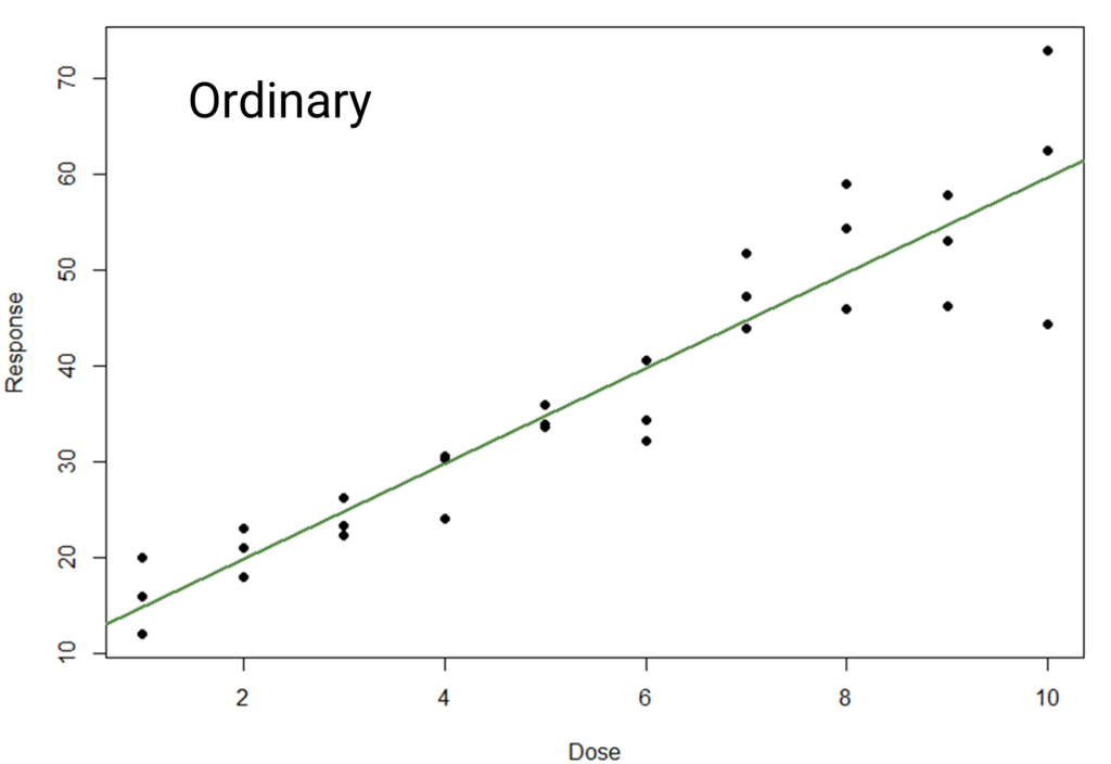
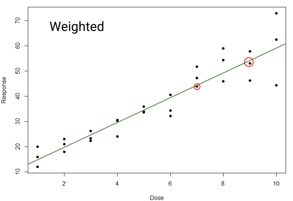
Below we have two model fits for the same data. First, we have an unweighted (or ordinary) fit to the data, and next is a fit weighted by the inverse of the variance.
The difference between the models here is small – try flicking back and forth between the images to see it more clearly. It is perhaps most visible near the top end, where the line is pulled closer to the points highlighted with the red circles. This is due to the high-response, high-variability points having less influence on the model, meaning the fit is “dragged up” less. While the difference is subtle, the weighted model will perform better when used for statistical inference.
Estimating Response Weights
While this method might theoretically produce optimal results, it is often difficult to apply in practice. Specifically, obtaining an accurate weight based on the dose group variance often requires an impractical number of replicates.
An alternative method of estimating weights is to find the relationship between the variances and the dose. Typically, if the variance of dose groups changes over the dose range, one can find a function which models the change. The weights can then be set as the inverse of the value of this function at each dose. That is, if the dose is given by x, and a function relating the variance of a dose group to the dose is f(x), then:
![]()
This method does not, however, represent a panacea. Arguably, it only moves the problem back a step as large amounts of historical data are required to find the relationship required with any kind of accuracy.
Weighting vs Transforming
As we’ve discussed several times on this blog, a different way to correct variance heterogeneity is to perform a mathematical transformation on the response values before fitting a model. In bioassay, a log transform is particularly common, but other transformations such as a square root transform are also useful in some circumstances.
The advantage of a response transformation over weighting is simplicity: compared to the complex statistical procedure required to calculate and utilise weights, a response transformation requires just a single mathematical operation. This means it is far easier to implement a response transformation and understand whether it has been effective at rectifying issues with homogeneity of variance, which, in turn, makes it a more accessible method for a non-statistician.
There are, however, occasions when a response transformation might not be appropriate. An example of this might be an assay whose linear range moves when a log or square root transform is applied. If not properly accounted for, this can lead to parallelism failures. Now, arguably the ideal solution in such cases would be to simply fit a 4PL model rather than a linear model. However, if this is not possible, then it might be necessary to consider weighting as a solution to heterogeneity of variance rather than a response transformation.
What do the regulators say about all this? The good news is that both are acceptable according to USP <1032>. Weighting receives more attention, but given the relative complexity of the two methods this is to be expected. And, in many cases, both choices give similar – if not functionally identical – results. As a general rule of thumb, we would recommend to first try a response transformation. Should that be ineffective, then consider a weighting-based solution. But, no matter what, always reach out to your statistician before moving forward with these decisions!


Comments are closed.