A Statistical Understanding of Polyclonality in Monoclonal Antibody Production

Therapies based on monoclonal antibodies (mAbs) are among the most powerful medical technologies to have been developed in recent years. From treatments designed to attack cancer cells and prevent rejection following organ transplants to methods for treating infectious diseases such as anthrax and COVID-19, the applications for mAbs continue to grow. And that’s before uses in diagnostics and assays such as the widely-used ELISA are included.

Antibodies are a key component of the immune system. They are proteins which bind to certain antigens – a different type of protein – on the surface of cells which are a threat to the body, such as cancer cells or pathogens. Importantly, antibodies are shaped to bind only with a certain antigen, or even just a specific part of a certain antigen known as an epitope.

In the human body, antibodies are produced by immune cells in the blood. To manufacture antibodies commercially, therefore, several technologies have been developed to clone such immune cells into artificial colonies from which the desired antibodies can be isolated. This also allows genetic engineering of the cells to produce antibodies which target a desired antigen.

If a colony is cloned from a single progenitor cell, then we say that the colony is monoclonal. Monoclonal antibodies are, therefore, those which are generated by a monoclonal colony. By contrast, if the colony is grown from two or more progenitor cells, then we say that it is polyclonal and it generates polyclonal antibodies.

The progenitor cell is engineered to produce antibodies which bind to a chosen target antigen, and since all the cells in the colony are identical to the progenitor, the mAbs produced will all bind to that antigen. This is important for the specificity of the produced antibodies binding to the target. That is, the ability for the antibodies to exclusively bind to the target. If the colony is polyclonal, there is an increased chance of antibodies which bind to other targets being produced, increasing the probability of false positive results.

While polyclonal antibodies have their own uses, such as for antivenoms, it is desirable to ensure that cell colonies are monoclonal when mAbs are being produced. While this requirement is not outlined in detail in regulatory guidance, it is suggested in documents produced by the FDA, EMA, and ICH that ensuring a high level of monoclonality is a basic expectation when producing mAbs.

As is so often the case with biologics, maintaining stringent quality standards is the primary motivation behind the need for monoclonality. A component of this is trying to minimise the variability in the critical quality attributes (CQAs) of the produced antibodies. As it turns out, antibodies from polyclonal colonies are more variable in quality than those from monoclonal colonies.

To understand this, imagine we have two groups of genetically-identical cells, group one and group two. These cells produce antibodies, for which we measure a property P, which we consider a CQA. Cells from group one always produce antibodies with P=1, and those from group two always produce antibodies with P=2.

If we had a monoclonal colony of cells from group one or group two, we would have no variability in our CQA. If, however, we had a polyclonal colony where we mix cells of group one and group two, then the range of possible outcomes is far greater – it could be one, two, or anything in between. The polyclonal colony produces antibodies of a far more variable quality than the monoclonal colony.

Now, this is a toy example with the effect deliberately exaggerated. In particular, we, of course, would never expect any real-world product to have no variability; even monoclonal colonies are subject to natural variation. We do, nevertheless, expect the product from polyclonal colonies to be more variable than that from monoclonal colonies. This is illustrated in Figure 1.

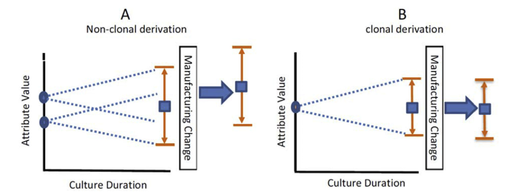
Notice how the range of possible outcomes “fans out” over time. This is a result of phenotypic drift – small changes in the genome of cells which result in differences in how they produce antibodies. While cell line stability studies typically form part of the mAb development process to minimise these changes, phenotypic drift, nevertheless, increases product variability over time for all colonies. It particularly exaggerates any differences between the multiple progenitor cells in polyclonal colonies.

A key part of mAb production, therefore, is screening cell colonies to detect inadvertent polyclonality. These colonies are typically grown in glass tubes, known as wells. Hundreds of these wells are seeded with single cells as part of the mAb development workflow. The natural cell division process then proceeds, resulting in a colony which produces antibodies.

Many of the wells fail and do not produce any antibodies. The wells which are successful in producing antibodies, however, are then screened and upscaled for further evaluation in biorectors. In an ideal world, all of these successful wells will have been seeded with a single cell, meaning the resulting colonies will be monoclonal. We refer to such wells as monoclonal.

Some of the productive wells, however, will have resulted from an incorrect seeding process: the well will have been seeded with more than one cell. This means that the product in the well will have derived from two or more genetic lines. We call such a well polyclonal.

Specialist equipment has been developed to ensure that as many wells as possible are seeded with a single cell for mAb production. It is, nevertheless, a requirement of many regulatory bodies that manufacturers estimate the proportion of their product which is monoclonal to ensure that high quality standards are maintained.

One way to estimate this proportion is a dual fluorescence experiment. Here, we undertake our seeding process with a stock of cells which express different fluorescent proteins. These are treated so they will fluoresce a given colour under UV light. Importantly, half the cells are treated such that they will fluoresce red, with the other half are treated such that they will fluoresce blue. One way this is done is through encoding the fluorescence onto the genetics of the cell, meaning that its colour will be maintained among the descendants of the progenitor cell. Other techniques, such as staining the cells using a fluorescent dye, are available, but we will focus on the genetic route here.

The purpose of the fluorescence is that, should a given well end up seeded with more than one cell, there is a reasonable chance – around 50% – that these starter cells do not fluoresce the same colour. That means that, while monoclonal cell colonies will always fluoresce the same colour, there is approximately a 50% chance that a polyclonal colony will contain cells which fluoresce different colours – or dual fluoresce – under a UV lamp. This allows us to determine that the well is polyclonal.

Now, some polyclonal wells – again, roughly 50% – will have been seeded with more than one cell which just happen to fluoresce the same colour. When we check these wells with the UV lamp they would not dual fluoresce, meaning we would falsely conclude that the well was monoclonal. This means that we cannot directly estimate the number of polyclonal wells, or, therefore, the probability of any one well being polyclonal, by simply counting the dual-fluorescing wells. We must, instead, turn to statistics.

A simple method to estimate the number of polyclonal wells in a given batch, employed by several authors, is to simply double the number of dual-fluorescence wells and use this as an estimate of the number of polyclonal wells. The thinking behind this is that if a polyclonal well has two cells, there’s a 50% chance those two cells will fluoresce the same colour, and a 50% chance they will dual-fluoresce. So, for every well we find that is dual fluorescing, there will, on average, be another well present that was seeded with two cells but does not dual fluoresce.

There are three problems with this approach:

1. Not every polyclonal well will have been seeded with exactly two cells. Some will have been seeded with three, four, or even more.
2. Not every cell will fluoresce as intended. A cell line which fails to fluoresce can make a polyclonal well appear monoclonal.
3. Our count is based on a sample. This means it is subject to the same uncertainties as any other statistical estimate.

The first two problems are addressed by a detailed probabilistic analysis of the seeding process. We list every possible polyclonal cell seeding scenario and determine the probability of each. This allows us to build up an estimate of the probability of a polyclonal well dual fluorescing. We can then use this to convert the number of dual fluorescing wells, which we can directly count using the UV lamp, into an estimate of the probability of monoclonality.

For now, we’ll focus on the case where the polyclonal well has been seeded with exactly two cells – we’ll define this as a 2-polyclonal well. Let’s say that a given cell has an 8% chance of being defective (i.e. it will not fluoresce even though it should), and that a red cell is as likely as a blue cell to be defective. This means the probability of a randomly chosen cell being a functioning cell of either colour is 46%, and the probability of being a defective cell of either colour is 4%. We also assume that the cells are all independent of each other – the fluorescence of any one randomly selected cell does not give us any information about the fluorescence of any other cell.

To calculate the probability of a 2-polyclonal well being dual fluorescent, we can enumerate all 16 possible 2-polyclonal wells and determine which combinations would be dual fluorescent. The probability of each combination can then be found using the outlined assumptions. This process is detailed in Figure 2.

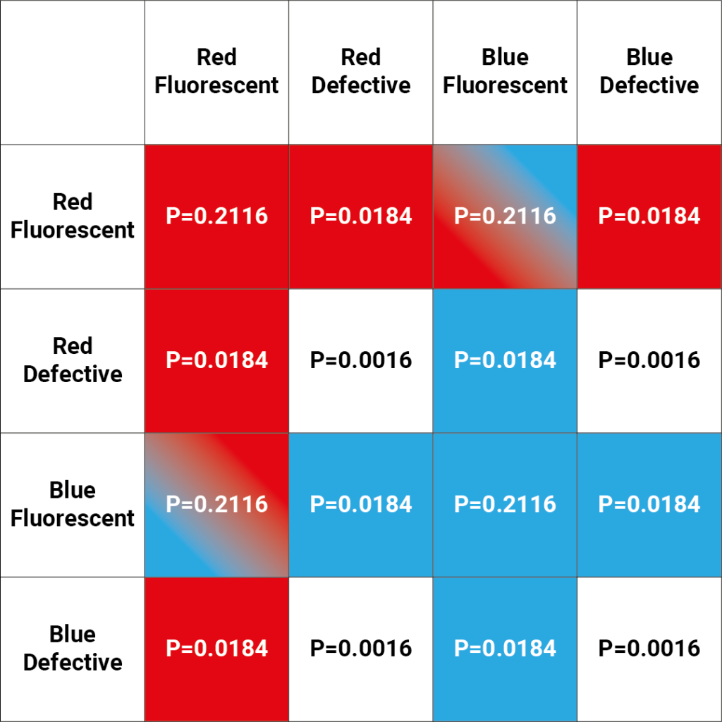
From Figure 2, we see that two combinations are dual fluorescent. Both require a red fluorescent and a blue fluorescent cell, so the probability of each is given by:

Since there are two possible combinations which produce a dual fluorescent colony, we mulitply this probability by two, which gives:

So, we find that the probability of a 2-polyclonal well being dual fluorescent is 42.3%. Note that the | is statistical notation for a conditional probability: means the probability of a well being 2-polyclonal given we observe it dual fluorescing under UV light.

We can perform a similar process for 3-polyclonal wells, which tells us that the probability of a 3-polyclonal well showing dual fluorescence is 68.6%. We could continue this process forever, calculating the probability of dual fluorescence for higher and higher order polyclonal wells. Due to specialist machinery and inspections during cell growth, however, it is highly unlikely that 4- or greater polyclonal wells will make it to the end of the growth process. We can safely assume, therefore, that the probability of a polyclonal well being higher order than three is zero.

Further, thanks again to the specialist machinery and monitoring, 2-polyclonal wells are far more common than 3-polyclonal wells. Let’s say that 95% will be 2-polyclonal, while 5% are 3-polyclonal. The overall probability of any polyclonal well dual fluorescing is then given by:

We call this value the k-parameter. Notice that our k-parameter is smaller than 50%. That means that using the commonly accepted method of doubling the number of dual fluorescent wells – effectively using a k-parameter of 50% – would overestimate the probability of a polyclonal well being dual fluorescent.

Let’s say that in our experiment we obtain 500 wells with successful colonies, and observe 8 – or 1.6% – that are dual fluorescing. Note that we’re only considering successful wells here: this would be a far smaller percentage of the total number of wells seeded. As with any statistical experiment, we should account for the sampling uncertainty in the number of dual fluorescing wells by calculating a confidence interval.

We recommend using the Clopper-Pearson or ‘exact’ method for generating confidence intervals in this case as it is the most conservative option. It gives us a 95% confidence interval of 0.7% – 3.1%. To remain conservative in our estimate of the probability of monoclonality, it is prudent to take the upper end of this confidence interval as the estimate of the probability of dual fluorescence.

Using this, we can conservatively estimate that 3.1% of successful wells will dual fluoresce in future runs. But, from our previous calculations, the k-parameter informs us that only 43.6% of wells which are polyclonal dual fluoresce. Thus, we need to inflate our estimate using the k-parameter. This is given by:

As all the wells that are not polyclonal are monoclonal, this means that our final estimate of the probability of monoclonality is given by

Had we instead operated under the naïve assumption that 50% of polyclonal wells dual fluoresce, we would have found that the probability of a well being polyclonal was 6.2%, meaning the probability of monoclonality would be 93.8% – an overestimate. While this may not seem like a serious issue, it is the kind of error which could push a batch of product from just failing to meet regulatory requirements to just meeting those requirements. This exposes the end user to increased risk of unintended consequences when using the produced mAbs.

It is, therefore, important to ensure that the correct methodology for estimating the probability of polyclonality is used. While it may be intuitive to simply use a k-parameter of 50%, even a shallow investigation into the statistics behind the dual fluorescence experiment reveals that the experiment has obvious complexities which ought to be accounted for. Including a statistician in the early stages of planning of mAb production is a good way to ensure a robust statistical methodology for polyclonality testing.