One of the most important metrics when analysing bioassay data is goodness-of-fit — how well does a dataset fit a chosen model? In development, this question can help determine which model is appropriate for a dataset, while new data will have to meet a goodness-of-fit criteria to ensure it is adequately represented by the chosen model to pass GMP requirements in routine analysis. What do we use to determine goodness-of-fit? We often see our clients using the coefficient of determination — more commonly known as R² — as a metric for goodness-of-fit for both linear and non-linear models. When asked at BEBPA Europe 2021, 35% of respondents told us they use R² for this purpose even for non-linear dose response models, such as a 4PL. Indeed, this is not a fluke. SoftMax Pro for bioassay analysis claims “The R² value is generally a good representation of the goodness-of-fit”.

All good then? Not so fast. In their 2010 paper, Spiess and Neumeyer beg to differ, stating “Researchers and reviewers should be aware that R² is inappropriate when used for demonstrating the performance or validity of a certain non-linear model”. Even SoftMax Pro can’t make its mind up, admitting—in the same blog post, no less—that “R² can be a poor measure of curve fit quality”.

There appears, therefore, to be some confusion on the question of whether R² is an appropriate measure of goodness-of-fit. From the title of this blog, you may have guessed where we at Quantics fall on the issue. We want to demonstrate why we think R² is a poor measure of goodness-of-fit regardless of model form: that a low R² doesn’t always indicate a poor fit, that a high R² doesn’t always indicate a good fit, and that R² doesn’t measure the shape of a dataset in the first place.

To examine why R² is a poor goodness-of-fit measure, we should first understand what R² is. In short, it is a measure of the strength of the relationship between a dependant variable (typically plotted on the y-axis) and an independent variable (usually on the x-axis). We’ll consider R² in terms of the variation of the y-value of data points. These are the vertical distances of the data points from a point of interest, such as the mean y-value of the data set or a fitted model curve.

A common formula for R² is:

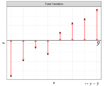
Let’s break this down. is the total variation of a dataset relative to its mean. As shown in Figure 1, this is equivalent to asking how close the y-values of each data point are to the mean y-value of the whole dataset. This value will be the same no matter what model we choose to fit to the data—it is model independent — since this variation is a property of the data itself, not of a model we impose.

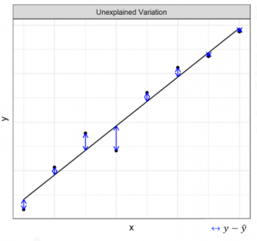
Conversely, residual variation, , does depend on our choice of model. Specifically, it measures the vertical distance of the points from the curve we fit to the dataset, which is shown in Figure 2. It is, in a sense, the variation which is “left over” when we fit a model to our dataset: that which is not “explained” by our choice of curve. And, since the distance between the points and the curve will change if the curve is changed—it is model dependent—the residual variation changes depending on which model we choose to fit.

R² takes the ratio of these two variations, and subtracts it from one. If we choose a model whose curve passes each data point exactly, there will be no residual variation (), meaning R² = 1. Conversely, if we choose the mean of the data as our model, then the residual variation will be identical to the total variation (), and R² = 0.

So, what does R² actually tell us? Recall our original definition of R²: a measure of the strength of the relationship between a dependant and independent variable.  If the relationship between the variables is strong, most of the variation in the data is explained by a best-fit model we impose, and R² is close to one. If the relationship is weak, however, then most of the variation is random noise in the data, meaning the residual variation will be large when we impose our model. This would result in a low R².

From our investigation so far, its easy to see why R² could be confused with a measurement of goodness-of-fit. One would expect a well-fitted model to explain most of the variation in a dataset, after all, and this is integral to the value of R². However, the connection does not hold in all cases. Far from it.

Take the two datasets shown in Figure 3. It is (hopefully) clear that these datasets are well-fit by the same linear model, which we can see in Figure 4. If R² was a measure of goodness-of-fit, we might expect these two models to have similar R² values.

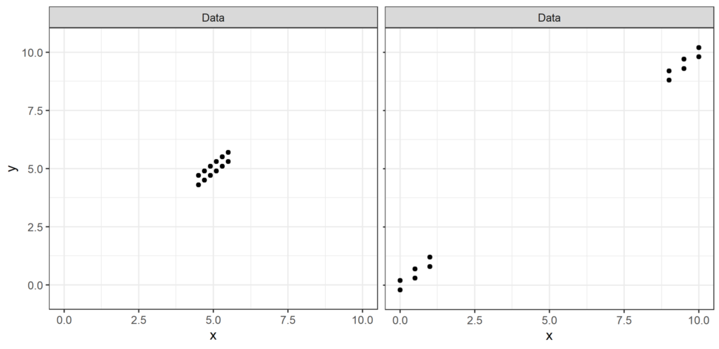
But do they? While the data in both sets lie close to the fitted curve, meaning that the residual variation () is small, the data in the left-hand plot is much closer to the mean (here = 5) than in the right-hand plot. This means that the total variation () for the plot on the left is much smaller, and, therefore, the ratio  is much greater. This results in an R² of 0.74 for the left-hand plot, while the R² of the right-hand plot—whose data lies further from the mean, resulting in a larger —is close to one.

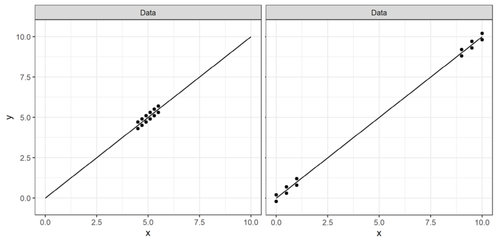
See the problem? Using R² as a goodness-of-fit measure, we’d surely reject the left-hand model with an R² as low as 0.74. But we can visually see that the model we’ve used fits the data very well, in fact near-equally well as the right-hand plot with an R² of close to one. While this is a single, constructed, example, it definitely shows that a low R² does not always indicate a poor model fit.

So, we know that R² is not a good measure of model fit at the lower end, but maybe a high R² is still a sign of a good model fit? The right-hand plot in Figure 4 has a R² close to one, after all, and we can visually see that’s a very good model fit. Sadly, even here, things are not that simple.

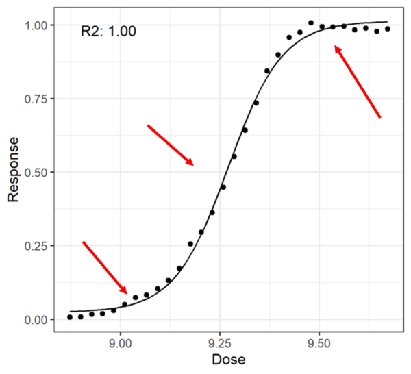
In Figure 5, a more complex dataset has been fit with a 4PL model. The datapoints are pretty close to the curve throughout, which means that will be small compared to . This results in a R² of close to one.

Again, we can see there’s a problem here. There are regions—indicated by red arrows—where the model is systematically a poor fit for the data. That is, the curve passes over or under several consecutive datapoints. For a good model fit, we would expect a more even distribution of points falling above and below the model curve over the full range of the data, as this is the pattern of variation more typically associated with random noise. Since there are systematic model fitting failures, it is easy to make the case that the model is not a good fit for the data despite the high R² value. Once again, then, we find that the R² value is not a good representation of the goodness-of-fit of the model.

A high R², then, tells us similarly little about the goodness-of-fit of a model as a low R². This leaves just one question outstanding: why? R² is a measure of how well a model explains the variation of a dataset so, intuitively, we might expect that it would measure goodness-of-fit.

The issue is that the variation is not the only important factor in goodness of fit: the shape of the data is also relevant. R² take this information about the shape of the data—in the total variation —and amalgamates it with information about the variation of the data around the chosen model—the residual variation . This combination is awkward to separate, and means that R² does not answer the all-important question of whether the shape of a dataset is matched well with that of a chosen model.

While R² may intuitively seem like a simple way to measure of the goodness-of-fit of a model, it is not the appropriate tool for the job. It is true that many well-fit models have a high R² value, while many a poorly fit model will have a low R², but this is coincidence. R² does not measure the shape of a dataset, which is the most important factor when determining goodness of fit. It is easy to concoct well-fitted models with low R² values, as well as poorly fitted models with a high R². To use R² as a metric for goodness-of-fit, therefore, is to not only risk unnecessary failures of perfectly good datasets, but also—and more concerningly—flawed datasets slipping through the cracks.

We hope that this blog has helped you to understand the problems of R². Choosing the best suitability criteria for your assay is not simple, and it is easy to end up with criteria that fail to perform as you expect, particularly when used in combination. Quantics is always happy to discuss system and sample suitability criteria choice, and this can usually be achieved with an analysis of development data. Doing this before it is all set in stone in commercial is a good idea!