Failing Goodness-of-Fit: How to Combat the F-test Headache
We have all experienced the frustration (and sometimes utter dejection!) of performing a bioassay to what you thought was near perfection only to come back, analyse the data, and find out your assay has failed goodness-of-fit. This can happen even when, visually, the data points look to be very close to the fitted model! What the F (test) is going on?!
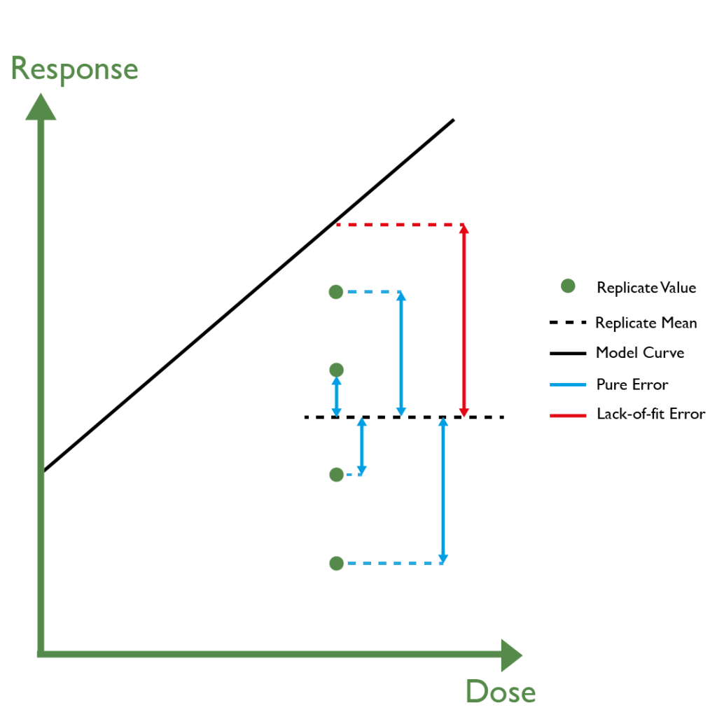
Unfortunately, this can be one of the maddening peculiarities of using the F-test to measure goodness-of-fit. As part of system and sample suitability testing, the F-test measures and compares the mean variability between the observed data and the model fit (lack-of-fit error), to the mean variability between replicates (pure error). This test essentially tries to determine two things – can the lack-of-fit error be attributed to the pure error, and if so, by how much?
Key Takeaways
- The F-test compares model fit errors to replicate variability. In highly precise assays, even small deviations can seem statistically significant, causing assays to fail goodness-of-fit unnecessarily.
- Averaging replicates and comparing model fits (e.g., 4PL vs. 5PL) can help determine if a simpler model is sufficient and reduce F-test sensitivity to trivial differences.
- Early use of individual replicates helps identify sources of variability. As automation improves precision, it is critical to reassess whether traditional tools like the F-test remain appropriate.
Why is my assay failing?
If your assay employs very good operator technique or advanced assay design including the use of liquid handling robots, the between-replicate variability (pure error) can be very low in comparison to the variability between the observed data and the model fit (lack-of-fit error). In circumstances where the lack-of-fit error is already quite small, the F-test will deem this small lack-of-fit error to be significantly high (due to the very low pure error), and the assay will fail goodness-of-fit, even though there are no evident flaws in design or technique.
The reverse can also happen where the F-test can accept a large lack-of-fit error if there is also large pure error; this will be considered insignificant, which will result in goodness-of-fit passing.
However, this is not what you want as there is a lot of variability in these situations, so it might not be a particularly good assay!
The smaller the pure error, the greater the influence of the lack-of-fit error on the F-test for goodness-of-fit. The result is a test that will “zoom in” on ridiculously small amounts of lack-of-fit error, consider that significant and fail the assay on goodness-of-fit.
Solving goodness-of-fit failures
One way to counter the “zoom in” effect of the F-test for goodness-of-fit is to constrain the p-value to a smaller significance value (e.g. 0.01 instead of 0.05).
This can, however, still cause unnecessary assay failures – for example, a validation project we worked on for a client had 23% of samples fail with a critical value of 0.05; when this was reduced to 0.01, 13% of samples still failed goodness of fit.
Another approach you could try (providing the between-replicate variability is consistently small during development), is to average individual replicates for each dose (concentration), so that you end up with one point per dose on your curve, rather than multiple points. Then analyse the data as follows:
- Fit the planned model and calculate the lack-of-fit error to the single data points.
- Fit a more complex model (e.g. 3PL if using linear, 5PL if using 4PL) and calculate the lack-of-fit error to the single data points.
- Statistically compare the lack-of-fit error from the planned model to that calculated for the more complex model.
- If there is no significant difference between the two, this means that the planned model is a good fit for your data, since adding a more complex feature does not improve the fit.
- If there is a significant difference between the two, this means that the planned model might not be the best fit for your data, and you should rethink the analysis method.
In most cases, averaging replicates will reduce precision (i.e. the confidence interval will be wider due to fewer data points being available for analysis). We recommend only trying this approach if your assay is already very precise to begin with, yet is still failing goodness-of-fit.
Most software packages should be able to statistically compare the lack-of-fit error. Our QuBAS software can absolutely perform this and much more!
Best practices
During the development stage/s of an assay, it is important to use individual replicate data initially, to observe between-replicate variability. This information is required to evaluate overall precision and inform the assay design with respect to numbers of replicates, plates etc. needed to achieve the required precision.
You should have a solid understanding of your assay design and the important sources of variability, along with good operator technique and performance.
Therefore, the approach outlined above is likely to be used in later development, once between-replicate variability has become consistently small.
You should keep in mind that averaging replicates will reduce assay precision – by how much depends on your early development information on replicate/plate numbers, closeness of between-replicate measurements, and so on.
Again, this approach should only be introduced when you know that the assay essentially has ‘precision to spare’ and is only failing goodness of fit.
This should always be performed before formal validation.
Goodness-of-fit failures are also something to think about when introducing more forms of high-end laboratory automation. The technology with liquid handling robots will only get better, resulting in an even finer degree of technical precision that will not be able to be matched by human operators. This may well raise the question of whether the F-test is even fit for purpose as assay variability becomes better understood and/or better controlled – but we will save this for another blog!
Quantics have considerable experience in using this approach as well as other methods to help avoid unnecessary goodness-of fit-failures, on otherwise well-designed and well-executed assays. Our QuBAS software takes the hassle out of analysing data, along with the confusion about which test statistic to select. Contact us to see how we can help you develop, validate or troubleshoot your assay.