USP <1033>: The Goals of Bioassay Validation

One can think of the life of a bioassay in two main acts. First comes the design and development of the assay, where the assay method is conceptualised, refined, and optimised. Later, the goal is for the assay to be deployed in a regulated environment to, for example, test batches of product to ensure that only those which meet the required specifications are released to patients. Between these two phases, however, comes a point of inflection: validation. This is the final hurdle a bioassay must jump to be deemed suitable for use in a GMP process. As a result, validation studies establish an assay’s performance, and can seem a long and daunting process for those at the start of the journey.

Our goal in this series is to provide a roadmap through the most critical steps in validating a bioassay. In doing so, we will follow along closely with the bioassay validation chapter provided by the United States Pharmacopoeia: USP <1033>. We’ve examined this chapter before, specifically to look at the changes in the upcoming revisions to the guidance. Here, we will take a wider view of the full chapter – while still incorporating those crucial changes – to provide a comprehensive guide to bioassay validation. This series will focus on validating assays used for making batch release decision, though many of the concepts here are applicable to validation of assays in other applications. In this first part, we take a broad view of a validation study, including its components and goals.

Bioassays are typically deployed in support of the manufacture of biologic drugs – a cell or gene therapy being an example. As with any product – particularly those used in a medical setting – batches of manufactured biologics must be tested against stringent specifications which ensure their safety and efficacy before they can be released for wider use. This is the role of a potency bioassay: to test that a manufactured lot is of the expected potency in order to protect end users from unsafe therapeutics.

But, how can we be confident that the bioassay provides reliable assessments of the product batch? Bioassays are, by their nature, highly complex and variable. If the release of a product is to hinge on a bioassay, then it is vital that we can trust the results provided by that bioassay so that the decision to release or scrap a batch of product is well informed. That’s where a validation study comes in. To validate an assay is to prove that it is able to provide results of sufficient accuracy and precision that can be used to support key product decisions. This is outlined in USP <1033>: “Assay validation is the process of demonstrating and documenting that the performance characteristics of the method underlying a procedure meet the requirements for the intended application and that the assay is thereby suitable for its intended use.”

Note that this means validation is different from a qualification or verification study. The goal of the latter studies is often to understand the performance of an assay so that acceptance criteria for a future validation study can be determined. A validation study, by contrast, aims to determine whether those criteria have been met. One might, therefore, perform a qualification study in advance of validation to inform the choice of acceptance limits, though this is not always required, for example, if sufficient historical data has already been collected.

As with so many aspects of pharmaceutical manufacturing, risk management is critical in validating a bioassay. This, critically, includes the mitigation of risk to the patient from unintentionally releasing an out-of-spec product, but also the risk to the manufacturer of misidentifying an in-spec product as out-of-spec. As we’ll explore in more detail, the accuracy and precision of an assay both affect the likelihood of an out-of-spec result, whether the product is truly out-of-spec or not. As a result, regulatory bodies require that assays used under GMP conditions – that is, those being used for testing products to be used in patients – be validated.

The most important outcome of a validation study is to determine whether the assay is suitable for its intended use. That means demonstrating that it is capable of providing results of sufficient accuracy and precision such that they are informative in the decision-making process surrounding a product, as well as ensuring the performance characteristics of the assay have been formally documented. These, of course, include the accuracy and precision, but also properties such as, linearity, and range.

Using Statistical Process Control (SPC) for Bioassays

Should I Average My Pseudo-replicates?

Defining a Statistical Analysis for Bioassay: Response Modelling

We have established that demonstrating the accuracy and precision of an assay represent key goals of a validation study. Before we proceed, therefore, we should establish what accuracy and precision are, how they can be quantified, and what they mean to your bioassay results.

Accuracy describes how close, on average, experimental results are to the “true” value of a parameter. Imagine we were weighing an object known to have a mass of 1kg. An accurate set of scales would return an average result close to 1kg. In contrast, an inaccurate set of scales would return a different average value – say 1.05kg. We would describe this second set of scales as biased.

Precision, on the other hand, describes the spread of repeated experimental results. A precise set of scales would return individual measurements that are ‘close’ together, say {1.01, 1.00, 0.99}. Whereas a set of scales with poor precision would return measurements that are ‘far’ apart, say {1.05, 1.00, 0.95}. When talking about assays, we often talk about the inverse of precision, variability or variance. The more variable an experiment is, the less precise it is, and vice versa.

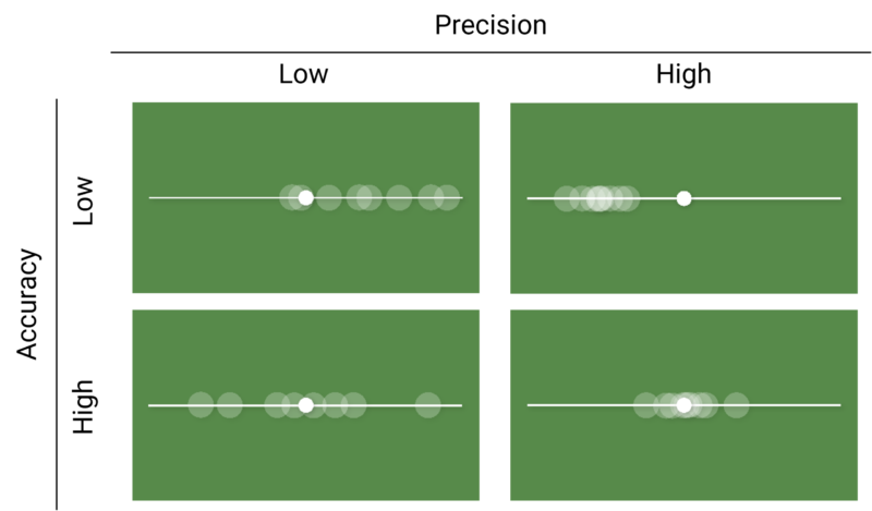
Crucially, the ability for an assay to produce good results depend on both its accuracy and precision. An accurate assay may not produce high quality results if it is horribly imprecise, and vice versa. Figure 1 shows a chart of images which outline this. In each image, the small white circle represents a “true” value, while the larger translucent circles represent experimental observations. We see that when precision is high, the observations are clustered close together regardless of whether that cluster is close to the “true” value – as in the bottom right image – or not – as in the top right image. Similarly, the “true” value falls roughly in the middle of the spread of the observations in both images where accuracy is high, representing the average result is close to the “true” value.

We can abstract the ideas of accuracy and precision further by thinking about the distribution of (repeated) measurements of the parameter we are interested in. In the context of bioassay validation this parameter would be relative potency, but it could also be the concentration of a sample in an ELISA. The distribution of measurements tells us about the probability of observing a particular value in an experiment: specifically, the area under the distribution curve between two values gives the probability of an observation falling between those values.

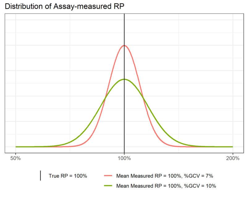
When we measure relative potency on the log scale, we find that it follows a normal distribution – we say that relative potency is log-normally distributed. Figure 2 shows two examples of such a distribution. We see that the curve is highest near the middle, and falls off steeply as we move to either side. This tells us that we are most likely to observe relative potency values near the middle of the range covered by the distribution, with that probability decreasing quickly (indeed, exponentially) as we move away from the centre.

We can define any normal distribution by two parameters: it’s mean () and its standard deviation (). The mean fixes the centre of the distribution – the average value – while the standard deviation describes the width of the distribution. The greater the standard deviation, the wider the distribution.

Now, recall that the probability of finding an observation in a range of values depends on the area under the distribution curve between those values. Definitionally, therefore, the area under the whole distribution must be equal to one due to the properties of probabilities. If this total area must be constant then, when we narrow the distribution, it must also get taller, meaning more of the area – and therefore probability – is located near the centre of the distribution. We can see this in Figure 2. The total area under both the pink and green distributions must be one, so the narrower pink distribution must be taller than the wider green distribution.

This property describes the connection between the precision of an assay and the standard deviation of its associated distribution. The standard deviation of the pink distribution is less than that of the green distribution, which is indicated by the pink distribution being narrower than the green distribution. This tells us that observations from the assay which produced the pink distribution are more likely to be closer to the measured mean – here 100% –those from the assay which produced the green curve. The former assay, therefore, is more precise than the latter.

In a bioassay context, we usually quantify precision using the Geometric Coefficient of Variation (%GCV). This is similar to the commonly used Coefficient of Variation (%CV), but is used when the measurement in question is log-normally distributed.  %GCV is defined as:

Where is the standard deviation of the log-transformed relative potency observations. is the base of the log scale on which the relative potency is measured. The choice of  is arbitrary – , , and (i.e. the natural logarithm) are common – but it is important to stay consistent once a choice is made.

In Figure 2, assuming we use the natural logarithm, for the green distribution. This gives us a %GCV of 10%. For the pink curve, , giving a %GCV of 7%.

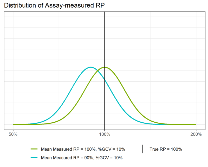
Similarly, the accuracy of the assay depends on how close the mean of the measured relative potency distribution is to the “true” relative potency value of 100%. In Figure 3, we see that the green distribution is centred on 100%. this means that the assay which produced these results has perfect accuracy – it is unbiased. Conversely, we see that the blue distribution is centred to the left of the true relative potency. Its mean is 90%, which means the assay is biased relative to the true relative potency and will, on average, underestimate the potency of the sample.

We quantify the accuracy of an assay using the Relative Bias (RB). This is defined as:

Where:

is the average relative potency measured by the assay

is the “true” or target relative potency

If an assay is unbiased, then the quantity (known as the recovery) will be one, meaning the %RB will be zero. If there is a difference between the average measured relative potency and the target potency, then the %RB will be non-zero. In the case of the blue distribution in Figure 3, the average measured relative potency is 90%, so:

We can, therefore, say that the assay which produced the blue curve shows a -10% bias at a target potency of 100%.

So far, we have given an overview of bioassay validation, including some common assay performance metrics and the overall study aims. In doing so, we described how demonstrating and documenting the accuracy and precision of an assay are among the key outcomes of a validation study. We’ve examined the definitions of accuracy and precision and built a framework relating these to the groundwork required for a deeper statistical understanding of the validation process. In the next part of this series, we will use the concepts described here to examine Probability of Out of Spec as a combination of the accuracy and precision of an assay, and how these feed into setting acceptance criteria for a validation study.