Using Statistical Process Control (SPC) for Bioassays

Bioassays serve as a method of testing a product: does the latest batch of our biologic have an acceptable potency? To do this effectively, we need to ensure that our test system – the assay – continues to function as it was originally designed. This is crucial as, in the worst case, a flawed assay could designate faulty products as acceptable, which could lead to potential harm to patients down the line. That’s why Statistical Process Control (SPC) is so important: it’s a method by which the behaviour of the assay system is monitored to detect problems and intervene before there is a chance of harm to the end user.

SPC is not a tool unique to the world of bioassay. Many of the concepts were first developed by Walter Shewhart at Bell Laboratories in the 1920s, and one of the first applications was in munitions manufacturing in the 1930s. Today, SPC techniques are used widely in industry and manufacturing, but also wherever frequent repeated processes are required, including, of course, routine bioassays.

Shewhart’s key insight was the idea of common and special causes of variation in the output of a manufacturing process. Common causes of variation are those which are expected to occur by natural variability in the process, while special causes of variation occur when something unexpected happens to change the output in some way.

For example, imagine you’re baking batches of cookies for a birthday party, and you’re trying to make sure that all the cookies are of similar size. We would expect a small amount of variation in the size of cookie due to, say, small differences in the amount of dough weighed out for each cookie, among other factors. These would be common causes of variation.

By contrast, a cause of special variation would be if your scales were miscalibrated, or if the butter in the mix was too warm resulting in cookies which spread unexpectedly. These issues in the manufacturing process would produce cookies with very different size to when everything was going to plan.

We say that manufacturing processes which are dominated by common variation are in control. Conversely, if special variation is present, this is a sign of something going wrong in the process, so we say that it is out of control.

The idea behind SPC is to give tests which help identify when special variation is occurring in the process, indicating it is out of control. This has the obvious benefit of flawed product being detected, but it also helps avoid unnecessary retesting or loss of product.

SPC enters the bioassay lifecycle when the assay has been validated: it is important that the assay is stable and not undergoing any changes in order to implement SPC techniques. This is because it is vital to establish the normal range of the attributes we wish to trend.

Once this is established, SPC can be used to detect any changes or drift in the assay characteristics. It is important that we spot if the assay behaviour has changed as this could be a sign that something has gone wrong – a sign we have special variation in the process and that it is out of control.

One example of a change which affects the behaviour of the assay is the degradation of the reference standard. As the reference ages, it will typically lose potency, meaning the measured relative potency of test samples will change. It’s important to monitor this shift as if the reference becomes too degraded it will need to be replaced. If the correct parameters are chosen, this can be monitored using SPC. For example, we might put checks on the EC₅₀ of the reference sample – as the reference sample’s potency decreases, the EC₅₀ will shift to the right.

Let’s imagine we have an assay which establishes the potency of a product ready for batch release. We’ve validated the assay, and we know that the data is well fit by a 4PL with a certain set of parameters. Let’s walk through the steps we would go through to set up SPC for this assay.

The first step in building an SPC process is to determine the key endpoints which will be monitored. These will typically be measurements of how the assay is performing, such as check on model fit and parameters. If we see these are out of control, this is a strong indicator that something has gone wrong in the assay.

It is, however, important not to choose too many endpoints. As with any statistical test, there is a chance that an endpoint is flagged as showing problematic behaviour due to random variability alone. The more endpoints we measure, the greater the likelihood of one of these chance failures, so the greater the likelihood of an unnecessary re-run or batch failure. It is, therefore, a good idea to measure the minimum number of endpoints which will still give you good coverage over the important properties of the assay.

Similarly, it is wise to avoid tracking endpoints which are strongly correlated. These are likely to pass and fail together, so we gain little extra information from examining more than one. Examples might include the assay range and both asymptote parameters – changes in one of these is highly likely to automatically imply a change in the other, so there is little point in tracking both.

Once we’ve chosen our endpoints, the next step is to determine how we want to track them in our SPC. The simplest method is to simply perform the SPC on the individual measured endpoint values for each sample. Alternative approaches are available depending on how the data is collected, such as data with some kind of inherent structure.

For our assay, we’ll keep it simple and look at the individual endpoint values. For an endpoint, we’ll look at the slope parameter of our 4PL model, which we’ll refer to as the B parameter.

Once we’ve established what we’re going to be tracking, the next question is whether our assay is under control for those endpoints. There’s little point in starting an SPC system on an assay which is already out of control, so we need to establish that we’re seeing a well-behaved assay by looking at historical data.

To do this, we calculate the mean () and standard deviation ()of a set of historical data for each of the parameters. We then establish alert and alarm limits for each parameter according to:

Alert limits:

Alarm limits:

These will be utilised throughout the SPC process.

Once the limits are established, we impose a set of rules to determine whether the assay is under control. There are several rulesets which one could apply at this stage, but all of them will be a combination of the following tests:

• How many values are outside the Alarm limits?
• How many values are outside the Alert limits?
• What’s the longest run of consecutive values entirely above or below the mean?
• What’s the longest run of consecutively increasing or decreasing values?

One ruleset using these tests was proposed by Oakland:

1. No values outside Alarm limits
2. ≤ 1 in 20 values outside Alert limits
3. No two consecutive values outside the same Alert limit
4. No runs or trends of ≥ 5 which also infringe an Alert limit
5. No runs of ≥ 7 entirely above or entirely below the mean
6. No rising or falling trends of ≥ 7

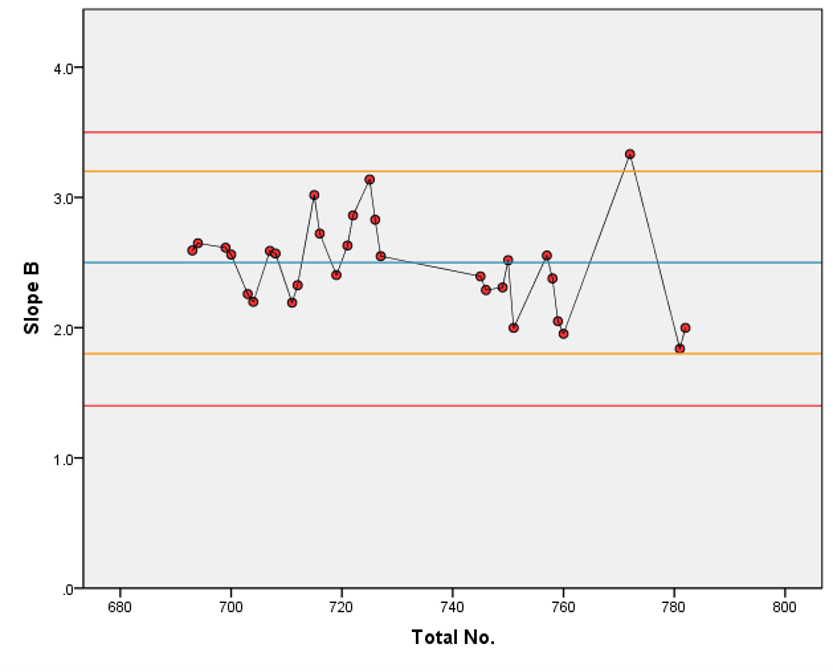
Let’s imagine we’ve already gathered some data for the B parameters of our model. What do our rules say about whether these parameters are in control? We’ve plotted the data, along with the alert (yellow lines) and alarm (red lines) limits on the graphs below.

On the left, we have the plot for the B parameter of our model. Applying our rules, we see that it passes on all 6, meaning we have good evidence that the B parameter is in control for this process.

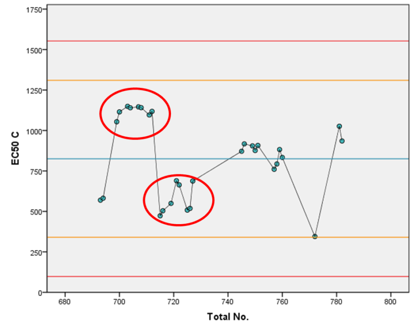
By contrast, on the right, we have data for the log(EC₅₀) (C parameter) of a different assay. We see that our rule concerning runs of ≥7 values above or below the mean (blue line) is contravened not once, but twice, which have been highlighted in red on the plot. This means that we would consider the C parameter as not in control in this process. We could, therefore, argue that SPC should not be applied to this assay as we have evidence that the process itself is not yet under control.

Once we’ve determined which parameter(s) we want to track in our SPC, the next stage is to set up control charts. These are plots – similar to the ones above – of sequential values of the parameters of interest produced in the assay. Now we have established that the assay process is in control, the idea is to check that it continues to remain in control by applying rules to the new data. There are several different sets of rules which can be applied here, such as Western Electric, Westgard, or Six Sigma. Here we’ll use Nelson rules, which are outlined below:

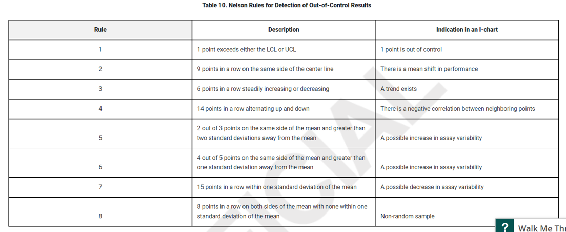
Every time we add a new data point to our control chart, we apply the rules to check whether we have evidence of the assay moving out of control. Let’s say we’ve begun to perform routine runs with our assay. The control chart below shows five additional B parameter values appended to the chart we used to show that the parameter was in control. The historical data is highlighted in green, while the new data is in blue.

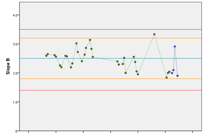
It is clear that none of our rules have been broken by any of these new data points, so we can comfortably carry on running the assay. Let’s imagine we run the assay for a few more days, and we end up with the below control chart.

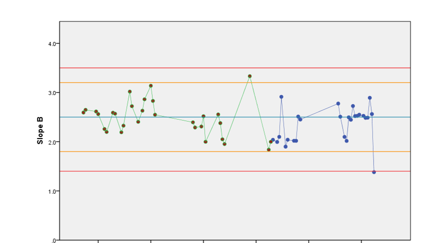
Now we have a problem! The most recent B parameter value has fallen outside our alarm limits, breaking the first of our rules. This is a sign that our assay could be moving out of control, so we should stop and investigate. We might, for example, re-run the assay with that day’s batch of product to check if this was just a chance result. If it isn’t, it might be a sign that something has changed in the assay system. This could be a known change, such as a switch two a different operator or even new pipettes, or it could be unexplained. In the latter case, this would likely require further investigation.

There will always be occasions when an assay is flagged by your SPC as a result of nothing but bad luck, particularly if the assay is monitored for a long period of time. Indeed, we can make a prediction of how often we would expect to see a chance failure. For normally distributed date, we expect 99.7% of data to fall within three standard deviations of the mean. That means we would expect approximately 1 in 370 observations to fall outside of this range. So, we would expect an average of about 370 assay runs before we saw a chance failure  due to a value falling outside the alarm limits. Other rules will give longer or shorter runs: the number of endpoints one is tracking will be a major contributing factor to this.

Nevertheless, it is important to continually evaluate the effectiveness of the rules you’re applying in your SPC. As Shewhart himself wrote in 1931, “the fact that the criterion which we happen to use has a fine ancestry in highbrow statistical theorems does not justify its use. Such justification must come from empirical evidence that it works”. The application of SPC and its rules are a useful tool, but be sure not to follow its lead blindly.

Implementing Statistical Process Control in bioassays is essential for maintaining assay integrity and checking that you get consistent, accurate results. Leveraging tools like QuBAS can streamline this process. QuBAS not only provides robust analysis capabilities but also allows you to easily export all assay data into SPC programs. This seamless integration enables effective monitoring of your assays, prompt detection of variations, and informed decision-making to keep your processes in control. By utilizing such advanced tools and adhering to SPC principles, you enhance product quality and reinforce patient safety and trust in your biologic products.