In our previous blog on survival analysis, we touched on some of the characteristics of survival data and various fundamental methods for analysing such data, focusing solely on non-parametric methods of analysis which only estimate the survival function at time points within the range of the raw data. I mentioned in the conclusion that parametric methods can be very useful for clinical trial research, as they can allow for extrapolation beyond follow-up.
Parametric statistics assume sample data is from a population which follows a particular distribution and has fixed parameters. Fundamentally, a model of the data is being created, which in turn can be extrapolated beyond the fixed follow-up time. Compared with non-parametric statistics, more assumptions are being made about a population. However if these assumptions are valid then inference could be more precise – e.g. standard errors of estimates such as median survival times will tend to be smaller [1].
This blog will explore the use of parametric methods to model survival data and extrapolate beyond given time points, using an example for illustration.
Key Takeaways
- Unlike non-parametric methods, parametric survival models assume a specific distribution and enable extrapolation beyond the observed data, which is critical in health technology assessments (HTAs) where trial data may be limited.
- The best-fitting parametric model is typically identified using a combination of visual inspection, log-cumulative hazard plots, and statistical criteria such as AIC and BIC.
- While extrapolated models can extend survival estimates, they are harder to validate without external data. Supplementary sources like patient registries improve reliability, and alternative methods such as piecewise modelling or hybrid approaches can also be considered for greater accuracy.
Modelling approaches
In the field of health technology assessment (HTA), data is usually censored or limited by short-term follow-up. If you limit estimation to only observed trial data, estimates of cost-effectiveness can be inaccurate [2]. For the economic evaluation of a treatment, extrapolation beyond the range of the data is needed to estimate the full survival benefit.
Parametric statistical models are commonly used, based on one of many distributions, including but not limited to:

The NICE Decision Support Unit Technical Support Document 14 (DSU TSD 14) [2] provides good guidelines for fitting the most appropriate model, which will be implemented in the following example.
To remain consistent with the previous blog, the “lung” dataset will be used in this example. To refresh your memory, this data consists of survival times of 228 patients with advanced lung cancer, split by sex, and the origin is the start of treatment. A snippet of data is shown below.
| Patient | Institution No. | Survival Time | Status | Sex |
| 1 | 12 | 1022 days | Censored | Male |
| 2 | 3 | 1010 days | Censored | Male |
| 3 | 15 | 965 days | Censored | Female |
| 4 | 1 | 883 days | Died | Male |
| 5 | 13 | 840 days | Censored | Male |
| 6 | 5 | 821 days | Censored | Female |
| … | … | … | … | … |
Modelling the survival curve
The NICE guidelines suggest three ways to compare different model fits to the data for a survival analysis.
1 Visual Inspection
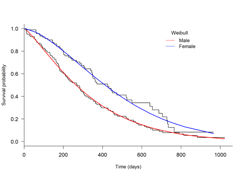
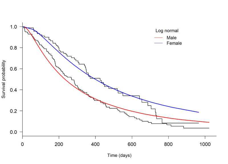
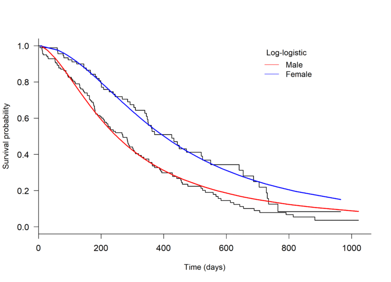
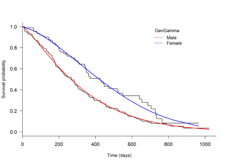
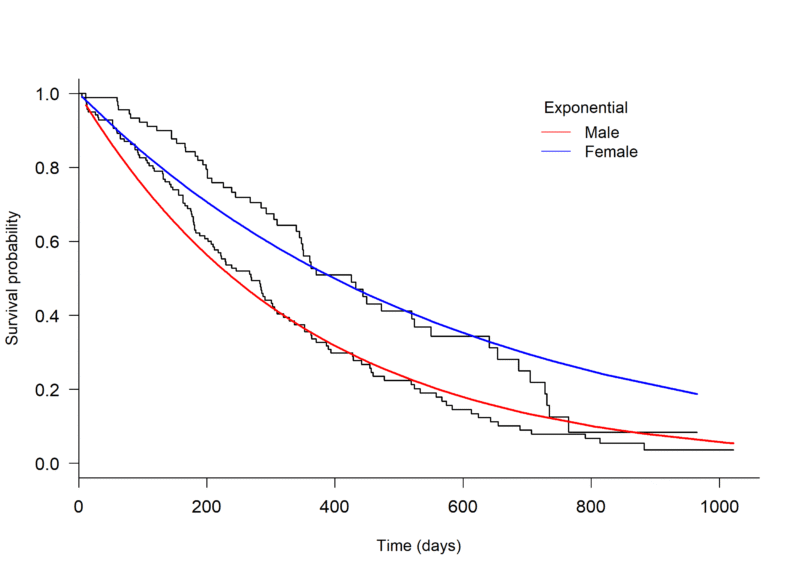
An initial assessment of model fit can be done through visual inspection, plotting a Kaplan-Meier curve to the survival data and overlaying with several parametric models. The plot.flexsurvreg function from the ‘flexsurv’ package in R can be used to fit different parametric models [4] (Figure 1, below).
Through visual inspection it appears as though the Weibull or Generalised gamma distributions fit the data best.
Figure 1. Kaplan-Meier plot of the Overall Survival of patients with advanced lung cancer, split by male and female, with parametric models fit seperately to each arm.
2 Log-cumulative hazard plots
The standard log-cumulative hazard plot [a] can also be used to assess suitability of an exponential or a Weibull model fit to the data. If the lines are straight, with slope = 1, an exponential distribution is a possibility. If the lines are straight but their slopes are not 1, the Weibull might be suitable [1].
Looking to Figure 2, the male arm appears to be roughly straight. The female arm has a large bend prior to day 60, following which it also appears straight. The large bend in this arm might be due to the data being sparse. The male and female arms have a slope of 1.1 and 1.3, respectively. The Weibull might be suitable model for both arms.
Figure 2. Log-cumulative hazard plot of male and female patients from the “lung” dataset, with time on the log scale.

3 AIC or BIC tests
The Akaike’s Information Criterion (AIC) and Bayesian Information Criterion (BIC) are statistical tests to compare models. These tests both penalise the use of extra parameters within a model. For example, a log normal model would be penalised more than an exponential model because it has an additional parameter. Extra parameters are penalised more by the BIC than the AIC. The model with the lowest AIC or BIC is considered to fit the model best.
Table 1 shows the AIC for each model, for each treatment arm (in this case sex; female and male) using the AIC function from the ‘flexsurv’ package in R, applied to the fitted models [3] (Table 1).
| Table 1. Akaike’s Information Criteria (AIC) of the male and female arms for the Overall Survival of patients with advanced lung cancer, for each model.
|
||
| Distribution | AIC (female arm) | AIC (male arm) |
| Exponential | 781.67 | 1537.52 |
| Weibull | 769.82 | 1532.34 |
| Log normal | 782.65 | 1549.77 |
| Log logistic | 774.24 | 1541.70 |
| Generalised Gamma | 771.49 | 1534.33 |
The Weibull model has the lowest AIC value for both males and females and therefore fits the data best compared to the other distributions. The results of all three assessments are consistent, and therefore the Weibull distribution is the most suitable choice to model the lung data.
Note: it is suggested in the guidelines to fit the same distribution to both treatment arms when fitting individual parametric models to each arm, as different distributions allow very different shapes and would require greater justification [2].
Extrapolating the model
The chosen parametric model can be extrapolated using the plot.flexsurvreg function from the ‘flexsurv’ package in R, specifying `t’, a vector of times to plot the fitted values from the model. The extrapolated Weibull model is shown in Figure 3.
In this plot the extrapolated curves are nearly merged by 1400 days. It would be best to provide external data to help support this result. Even in the absence of external patient-level data, summary statistics from a patient registry can provide useful information to improve accuracy. For example, the percent survival at a certain time point beyond follow-up can give insight to whether or not the extrapolated curve is reasonable, i.e. whether percent survival of the extrapolated portion closely compares the external data [2].
Figure 3. Kaplan-Meier plot of the Overall Survival of patients with advanced lung cancer, split by male and female, with parametric models fit separately to each arm and extrapolated beyond the follow-up time.

Limitations and considerations
When using a parametric model to extrapolate a survival curve, it is important to remember that there are limitations to assessing the model fit. You can test the fit of a parametric model to the available data, but it is difficult to assess the fit of the extrapolated portion without the use of external data. That being said, if there is a large amount of clinical data or there is minimal censoring, it might be reasonable to assume that a parametric model that fits the data well will also extrapolate the data well [2]. However when there is a high proportion of censored times, it is not always reliable to make this assumption. In any case, external data and/or clinical validity can be used in addition to the patient level data to improve extrapolation [2].
Other methods of extrapolation exist and have been implemented in a few health technology appraisals for NICE, including the LRIG Exponential method and Gelber method. Both of these methods are a combination of non-parametric analysis of the observed data and parametric analysis of the extrapolated portion. Further information on these methods can be found in the NICE TSD 14 [2].
Piecewise modelling is a more flexible parametric modelling approach. It can be valuable when fitting to data with variable hazards over time, as a model is fit to different time periods rather than fitting one model across the entire time period. When fitting this model it is important to choose time periods carefully, as not to choose a time too close to the tail-end of the data because there is greater chance of uncertainty. It would also be wise to consider external data when fitting this model.
Conclusion
Parametric modelling is common practice in clinical trial research, particularly in health technology assessment. It allows for a survival analysis curve to be extrapolated and parameters such as survival benefit to be estimated beyond the follow-up time. NICE DSU TSD 14 [2] is a useful and easy-to-follow guide for fitting and extrapolating these models. Furthermore, it is important to consider the use of external data for survival modelling to improve extrapolation, especially when the data is sparse. External data was not covered in detail in this blog. However it is an important topic for discussion, so stay tuned because it will appear in one of our future blogs.
References
[1] Collett, D. (2015). Modelling survival data in medical research. CRC press.
[2] Latimer, N. (2011). NICE DSU Technical Support Document 14. Survival Analysis for Economic Evaluations Alongside Clinical Trials – Extrapolation with Patient-Level Data, Sheffield, NICE Decision Support Unit.
[3] Therneau, T (2015). A Package for Survival Analysis in S. version 2.38, URL: https://CRAN.R-project.org/package=survival.
[4] Christopher Jackson (2016). flexsurv: A Platform for Parametric Survival Modeling in R. Journal of Statistical Software, 70(8), 1-33. doi:10.18637/jss.v070.i08
[a] Log-cumulative hazard plot; log(-log(S(t))) vs. log(t)




Comments are closed.