
Survival Analysis for Clinical Trials
We have discussed Handling Missing Data in Clinical Trials elsewhere, and mentioned a kind of missing data known as ‘censoring’. In this blog we focus on techniques for dealing with this, known as ‘Survival Analysis’.
Censoring occurs in time-to-event data (the time from a defined origin until the event of interest), when the event has not been observed (i.e. the time to the event is unknown). In a clinical trial, the origin might be randomisation or the start of a treatment, and the endpoint of interest might be disease diagnosis, the occurrence of an adverse event, disease progression, or even death. The key attribute of this kind of missing data is that the time to the event is partly known – it is at least as long as the event-free period observed for the subject – in other words, it is censored. This type of data can be analysed with a set of techniques known as ‘Survival Analysis’ [1].
Key Takeaways
- Survival analysis addresses time-to-event data where censoring occurs if the event has not been observed.
- Right censoring (event after study end or loss to follow-up) is the most common type in clinical trials.
- The Kaplan–Meier estimator provides a non-parametric estimate of the survival function and group differences can be assessed with the log-rank test.
- Parametric approaches (including Cox proportional hazards and fully parametric models) enable extrapolation beyond the study period for long-term effects.
To illustrate time-to-event data and the application of survival analysis, the well-known lung dataset from the ‘survival’ package in R will be used throughout [2, 3]. This data consists of survival times of 228 patients with advanced lung cancer. The origin is the start of treatment.
Types of censoring
Data can be either right, left or interval censored. In each situation the subject commences the study at a defined time to and the event of interest takes place at to + t. However when t is unknown and the event is only known to have occurred at to + c, the data is censored with a censored time, c.
Right censoring is the most common, occurring when the true event time is greater than the censored time, when c < t. It often arises when the event of interest has not occurred by the end of study and the subject has been lost to follow-up.
Left censoring is the opposite, occurring when the true event time is less than the censored time, when c > t.
Interval censoring is a combination of left and right censoring, when the event time is known to have occurred between two time points: c1 < t < c2.
Figure 1 illustrates the recurrence of lung cancer in three patients who received surgery to remove the tumour, indicated by the ‘start of study’, each patient depicting a different type of censoring.
Interval censoring can be observed at point A. This patient was examined at 3 months following surgery and observed to be disease-free. When re-examined at 6 months, the cancer returned and thus the actual time of recurrence is only known to have occurred between 3 and 6 months.
Left censoring can be observed at point B. This patient was examined at 3 months following surgery and the cancer had returned. The patient had not yet been observed disease-free and it is only known that the tumour returned sometime before the 3 month examination.
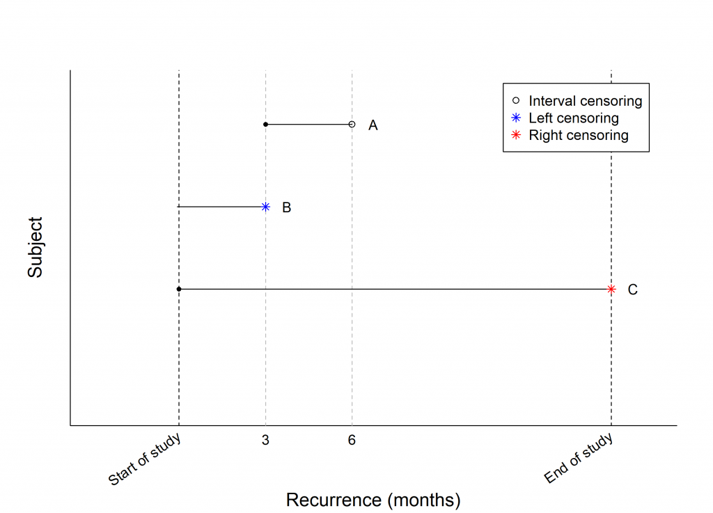
Right censoring can be observed at point C. This patient reached the end of the study disease-free but was lost to follow-up, therefore the actual time of recurrence is only known to be sometime following the end of study.
What basic information is required to perform analysis?
The most common type of censoring in clinical studies is right-censoring, and we will focus on this for the remainder of this blog.
For analysis, time-to-event data should consist of two pieces of information for every observation:
- The time to the event, or censoring time
- The event status (whether or not the event occurred).
With this information, a key function can be used to summarise the data and visualise the distribution of event times – the survival function.
What is the survival function?
The survival function can be defined as the probability that an individual survives past some time t, or similarly the proportion of patients still alive at time t, given by
\(S(t) = P (T \geq t)\),
where t is the actual survival time and T is a continuous random variable.
A widely used method of estimating S(t), and usually one of the initial approaches to analysing censored survival data, is the Kaplan-Meier estimator. This is denoted by \( \hat{S}(t)\). In clinical trial research, this estimate is often used to measure the proportion of subjects still alive at specified time points following treatment. Suppose the observed times of death in the study are t1, t2,…,tk with di deaths occurring at ti and ni patients alive just prior to ti. Then \( \hat{S}(t)\) is estimated by,
\(\hat{S}(t) = \prod_{i=1}^{t_i \le t} \bigg( \frac{n_i \, -\, d_i }{n_i} \bigg)\)
(Note that if a patient is censored at a time ti, they are included in ni, but excluded from ni+1.) The Kaplan-Meier estimate can be visualised through a plot of \( \hat{S}(t)\) versus t known as a Kaplan-Meier curve.
In practice, the ‘survfit’ function in the Survival package in R can be implemented to calculate Kaplan-Meier estimates and other important parameters, and produce the corresponding Kaplan-Meier curve [2].
Example
This ‘survfit’ function was applied to the lung dataset in R. A summary of the resulting Kaplan-Meier estimates at various time points are provided in Table 1 and the Kaplan-Meier plot is provided in Figure 2.
Interpreting the results
As shown in Table 1, the estimated probability of survival 208 days following treatment is approximately 0.66, i.e. 66% of patients are still alive; 138 patients are still at risk and 1 patient died. The estimated probability of survival is also shown in Figure 2, where the plot line falls on the intersection of 208 days and overall survival of approximately 0.7.
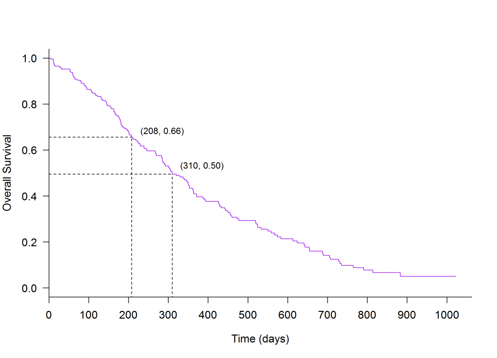
In practice it is often of interest to measure the median death time, or the time at which 50% of patients have died. This can easily be derived from the Kaplan-Meier curve by finding the time on the x-axis that corresponds with an overall survival of 0.5 on the y-axis. In this example the time at which 50% of patients have died is approximately 310 days following treatment.
Table 1: Kaplan Meier estimates
| Time (days; ti) | No. at risk (nj) | No. of events (dj) | \(\hat{S}(t)\) |
|---|---|---|---|
| 0 | 228 | 0 | 1.0000 |
| 5 | 228 | 1 | 0.9956 |
| 11 | 227 | 3 | 0.9825 |
| 12 | 224 | 1 | 0.9781 |
| … | … | … | … |
| 201 | 144 | 2 | 0.6708 |
| 202 | 142 | 1 | 0.6661 |
| 207 | 139 | 1 | 0.6613 |
| 208 | 138 | 1 | 0.6565 |
| 210 | 137 | 1 | 0.6517 |
| 212 | 135 | 1 | 0.6469 |
| 218 | 134 | 1 | 0.6421 |
| 222 | 132 | 1 | 0.6372 |
| … | … | … | … |
| 305 | 87 | 1 | 0.5129 |
| 306 | 86 | 1 | 0.5070 |
| 310 | 85 | 2 | 0.4950 |
| … | … | … | … |
Comparing survival for groups of subjects
In clinical trial research it is often of interest to compare two groups, such as comparing a treatment group to a control group. The log-rank is a hypothesis test for right censored data, which tests for a difference in the outcome between two groups of individuals. This test can be carried out using the function ‘survdiff’ in the Survival package in R [2].
Example
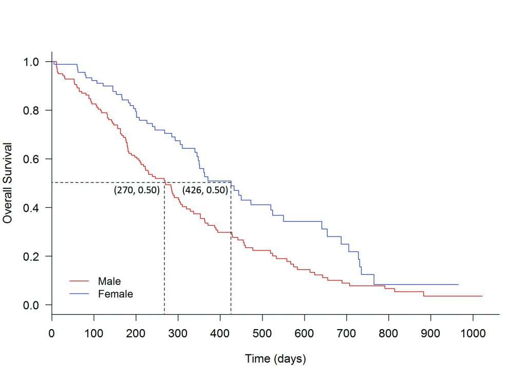
The lung dataset was grouped by sex.
Log-rank test
The ‘survdiff’ function was applied to the lung data, and the conclusion is that there is a significant difference between male and female treatment groups, with a p-value of 0.0013.
One way to summarise the difference is by comparing the median survival for the groups. The median survival for males was estimated to be 270 days and for females it was 426 days.
Where does this lead?
The method that was discussed here for estimating the survival function is non-parametric and only estimates the survival function at time points within the range of the raw data. There are many other approaches including Cox’s Proportional Hazards model, and fully parametric models.
In addition, it is often important in clinical research to understand the long term effects of a treatment, beyond the time-scale of a clinical trial. This places importance on parametric methods, which can be used to model the available data and extrapolate beyond the end of study, estimating the probability of an outcome over a longer period of time. These methods are common in practice and therefore they will be the topic of discussion in a future blog.
References
- [1] Collett, D. (2015). Modelling survival data in medical research. CRC press.
- [2] Therneau T (2015). A Package for Survival Analysis in S. version 2.38, https://CRAN.R-project.org/package=survival.
- [3] Loprinzi CL. Laurie JA. Wieand HS. Krook JE. Novotny PJ. Kugler JW. Bartel J. Law M. Bateman M. Klatt NE. et al. Prospective evaluation of prognostic variables from patient-completed questionnaires. North Central Cancer Treatment Group. Journal of Clinical Oncology. 12(3):601-7, 1994.