Statistical Sample Size Calculations for Clinical Trials

When scientific a study is evaluated, the sample size is often among the first issues brought up. Whether it’s the number of participants in a study, the number of times an experiment is run, or even the number of people asked to complete an electoral poll, it is well-known that – in general – a larger sample size means a greater chance that the study will return a result which is representative of reality.

In almost all cases, however, a greater sample size means greater costs to running an experiment. This is certainly the case when running a clinical trial. We usually want to include as many participants as possible, but each additional patient in the trial means another fee to a hospital to cover procedures and testing, added complexity for administration and logistics to ensure the correct treatment is delivered and its results recorded, and much more. This means that the study size is often among the most significant factors in the cost of a clinical trial to the sponsor.

That means there are two competing interests at the heart of every clinical trial: the need for the study to include enough participants to provide a robust result, and the desire of the sponsor to minimise the cost of the trial. As a result, one of the most important stages of preparing a clinical trial protocol is a sample size calculation, with a goal to determine the minimum possible number of trial participants while still allowing a functional study to take place. This is tightly controlled by regulators: most require that a study protocol includes a justification of the sample size.

To make a decision about an optimal sample size for a clinical trial, we must first understand the anatomy of the experiment. In most cases, this takes the form of a hypothesis test.

Many clinical trials compare a new treatment to the current standard of care. To set up the experiment, we first specify the null hypothesis, generally denoted by . This is usually the status quo – in this case, that the new treatment is no better than the current treatment.

We also specify an alternative hypothesis, or , which is usually the result a sponsor wants. Here, it would be that the new treatment is better than the current treatment. If properly defined, it should be the case that exactly one of and is a true representation of reality. We usually think of our hypotheses as examining the difference between the mean response () in each treatment group. This difference is known as the treatment effect, or often just the effect. In a case where a larger mean response is seen as better, this would mean the hypotheses are:

Note that, here, we are looking at a one-sided hypothesis test: we care about the direction of the effect. If we wanted to determine whether the new treatment had any effect at all – positive or negative – we would use a two-sided test, meaning our hypotheses would have a different structure.

Once we have gathered data, we can calculate the treatment effect, and consider our results. If we have evidence to show that the new treatment is indeed better than the current treatment, then we reject the null hypothesis and accept the alternative. Conversely, if this evidence is not apparent, then we fail to reject the null and conclude that the new treatment has failed to demonstrate that it is superior to the current treatment. Note the specific language here. Failure to reject the null is not equivalent to a conclusion of the null being true. Absence of evidence is not evidence of absence: it is possible that the null is indeed false, but the experiment was unable to provide evidence for that conclusion.

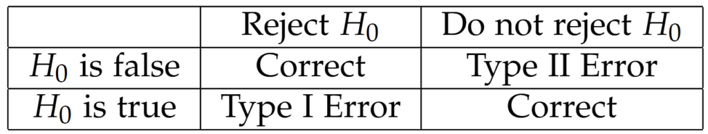
At the end of our trial, we will either reject our null hypothesis and accept the alternative, or we will fail to reject the null. We must base these conclusions only on the evidence provided by the trial. It’s possible that reality differs from our conclusions. The four possible outcomes from a hypothesis test are outlined in the table below:

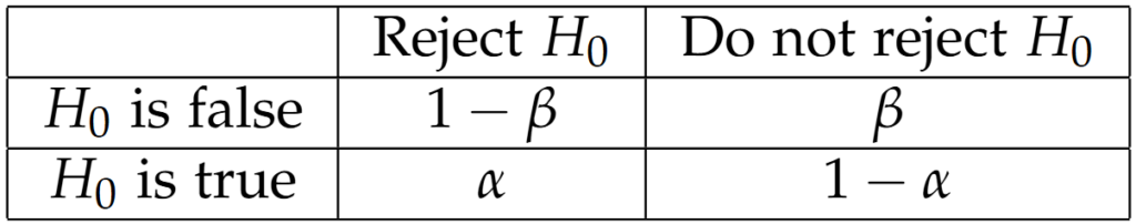
For every hypothesis test, there will be a probability of a Type I or Type II error. These probabilities are typically referred to as and respectively.

is the probability that the study will find that the new treatment is effective by a pure quirk of variability. is set by the sponsor at the start of the study – a standard choice for a one-sided test is 2.5%, while the standard choice for a two-sided test is 5%.

Another important probability is the chance that we will correctly find that the new treatment has a significant effect – that is, we reject the null, and the null is actually false. The probability of this outcome is known as the statistical power of the trial.

Mathematically, the power is defined as . In the case where is false, we have only two possible options: either we come to the correct conclusion and reject the null, or we make a Type II error. Probabilities are unitary – they must add to one – so, with the probability of making a Type II error defined as , we find the probability of drawing a correct conclusion to be .

The statistical power of a trial depends directly on the sample size, as well as several other factors including the size, distribution, and variability of the underlying effect. If, therefore, we specify a target power for our trial – specified as 80% by most regulators – the sample size required to achieve that power can be calculated under a set of assumptions made about the behaviour of the effect.

Let’s take a look at the distributions which outline the probability of obtaining a particular result from a clinical trial. Figure 1 shows an example: for simplicity, we’ve assumed the endpoint follows a normal distribution. The area under any region of the distribution represents the probability of the measured result falling between the limits of that region. Note that we do not know anything about these distributions absolutely. Their properties – mean, standard deviation, etc – must be estimated from the experiment or fixed by assumption.

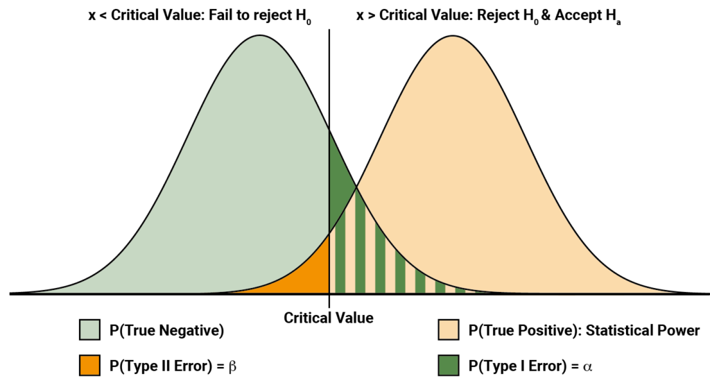
Notice that we have here two distributions. The left distribution represents the distribution of possible measured effects given is true, while the right distribution is distribution of possible measured effects given is true. The vertical line represents the critical value for the experiment: if the result falls to the left of the line, we fail to reject , while if it falls to the right we accept . The dark green shading represents the probability of a type I error – . Similarly, the dark orange shading represents the probability of a type II error – .

The statistical power is represented by the pale orange shading. From this, we can gain an intuition for why the statistical power is defined as . The area under any full probability distribution must equal one, so the total area of the dark orange and pale orange regions must equal one.

The underlying distributions are tied intrinsically to the properties of the effect and the experiment. For example, the effect size controls the shift between the two distributions. If the effect size is larger, then the right distribution moves further to the right. All else remaining unchanged, pale orange area increases, meaning the statistical power is grows. This is shown in Figure 2 (Top).

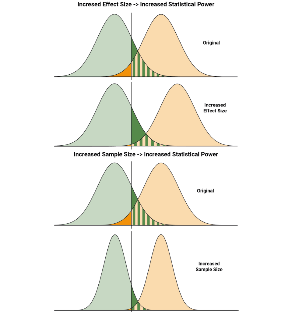
Increasing the sample size decreases the variability in the experiment by, for example, reducing sampling error. This narrows the distributions, once again meaning the pale orange area grows and the statistical power of the trial increases. This is shown in Figure 2 (Bottom).

So, what are the stages a statistician works through to estimate an appropriate sample size for a clinical trial?

It is impossible to begin estimating a sample size without first determining the hypotheses which will be tested by the clinical trial. These require input from the sponsor to define. For example, either a non-inferiority or a superiority margin needs to be decided. This is the effect size between the two treatments which is considered clinically significant and cannot be determined by the statistician. Common margins are the minimal clinically important difference or zero, but the decision is ultimately arbitrary and in the hands of the sponsor. Similarly, the choice of and target statistical power are to be made by the sponsor, but these are often informed by recommendations from regulatory guidances.

Once the framework of the test has been outlined, the next stage is to gain an understanding of how the statistics of the experiment is likely to behave. This includes such things as the distribution the results are likely to be drawn from and the variability of the results. Both of these factors, among others, will affect the optimal sample size. This stage is largely in the hands of the statistician, but is informed by previous experience of developing and testing the treatments from the sponsor. Many of the decisions at this stage will be assumptions based on the information provided.

As previously discussed, the appropriate sample size can be calculated based on the chosen target power and , along with the assumptions made about the behaviour of the endpoint in question. The goal is to find the minimum sample size which gives the required target power.
There are multiple ways this calculation can be done. Specialist software for power analysis and calculating sample sizes exists, such as PASS. Many more general programming environments also have sample size calculations, such as pwrss in R.

An alternative approach involves simulating the study under the choices and assumptions made. This allows the minimum sample size to achieve the desired power to be predicted. A simulation approach is often more time consuming and resource intensive than using an approach which directly calculates the sample size, but can be necessary in a case where a particularly complex statistical test is used for a study.

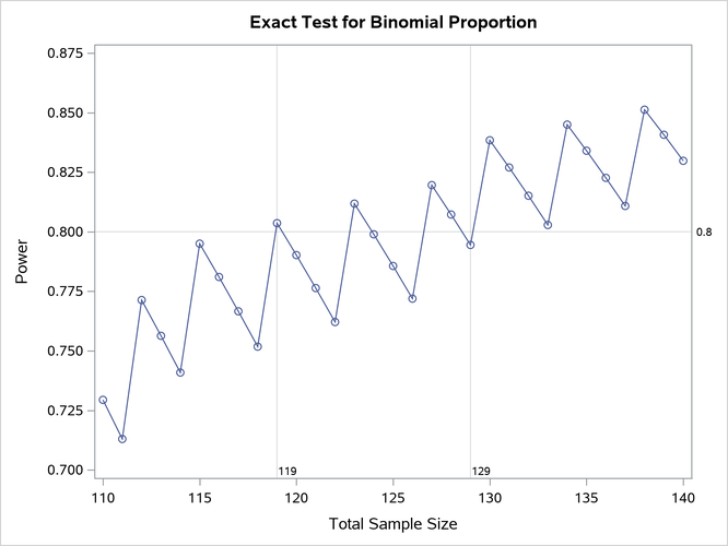
While the principle of a larger sample size giving a greater statistical power holds in most cases, there are some endpoints where one must be careful of the “sawtooth effect”. For binary endpoints, it is possible that a small increase in sample size can result in a decrease in study power. This is shown in Figure 3. In such situations, the recommended sample size should be the minimum sample size for which the target power is achieved and for which no higher sample size fails to achieve the target power. This is to prevent a case where the study ends up underpowered by a small overshoot on the study sample size.

It is highly unlikely that all the data which could have possibly been analysed in a clinical trial will eventually end up under the statistician’s knife. Subjects regularly leave trials for a variety of reasons, and it is common for data from some of those who remain to go uncollected or be unanalysable. To statisticians, all such cases are known as dropouts: data which is no longer available for analysis, for whatever reason.

It is important to account for these dropouts when deciding the final sample size for a clinical trial. If instead the bare minimum sample size which achieves the target power is used, then any dropouts would leave the study underpowered. The final stage of calculating a sample size for a clinical trial, therefore, is determining the dropout-inflated sample size.

To do this, the projected dropout rate is determined by the sponsor. The dropout-inflated sample size (DISS) is then calculated as:

Note the formula used here. A common error is calculating the new sample size using . This is incorrect, and underestimates the sample size required to account for the expected dropouts. This underestimation is particularly egregious if the dropout rate is high.

As we’ve outlined, the process of deciding on an optimal sample size for a clinical trial involves input from both the sponsor and the statistician. The calculation also involves several assumptions about the data and its variability which affect the final result. It is, therefore, important for the sponsor to have a good understanding of the trial – along with an understanding of the literature surrounding comparable products and the therapeutic area – before looking to determine a sample size. This gives the statistician the capacity to perform a well-informed calculation and determine the optimal sample size.