Driving Below the LOQ: Statistical Analysis of Unquantifiable Data

In many fields of science, researchers often face the challenge of measuring extremely small quantities. The life sciences are no exception, with experiments regularly requiring accurate and precise detections of tiny concentrations of impurities or other substances. Even while analytical techniques have advanced, manufacturing processes have improved in lockstep, meaning the capabilities of the testing infrastructure continue to be pushed. That means researchers and statisticians are regularly confronted with measurements which fall below the limit of detection (LOD) or limit of quantitation (LOQ) of an experiment. Here, we’re going to examine commonly used approaches to conducting a statistical analysis when collected data falls below the limits of what can be reliably measured.

Even the most advanced experiment will have a limit to what it can measure. No clever setup or computational algorithm can overcome the laws of physics. That means that every experiment will have a limit of detection, or LOD. This is the smallest quantity which can be detected by an experiment at all. For example, the LOD for a classroom ruler might be the smallest length you could see with your naked eye – it’s impossible to compare the length of an object to the scale on the ruler if you can’t see the object in the first place!

An experiment’s limit of quantitation, or LOQ, is more nuanced. The experiment can detect that something has been detected, but it cannot quantify that something with acceptable accuracy and precision. The LOQ for a ruler would be the distance between the marks on its finest scale (e.g. 1mm on most rulers in the UK). A measurement of an object smaller than 1mm will still return a result – i.e. a length of <1mm – but this result will not be as accurate and precise as a measurement of an object whose length falls above the LOQ. Experiments can have both an upper and a lower LOQ – a measurement might be so large that it saturates a detector, for example.

For an assay, the LOQs are defined as range of concentrations of an analyte which can be measured with acceptable accuracy and precision. An ELISA, for example, is most precise when the measured response of a test sample falls in the linear portion of the standard curve. If the response falls near the upper or lower asymptotes, the precision of the measurement decreases noticeably. If a sample returned responses which all fell on an asymptote – say if its concentration was so low that all measured responses fell on the lower asymptote – it may be the case that the precision of the interpolated concentration was not acceptable. This would mean that concentration would fall outside the lower LOQ of that ELISA.

A measurement which falls below the LOD of an experiment returns no data, so these cases are not of statistical concern. Measurements below the LOQ, however, still provide usable data. It falls, therefore, on the statistician to recover as much information as possible from such measurements. We’re going to examine two methods for doing this, and evaluate which provides the more useful results.

An incredibly simple approach to utilising data which falls outside an LOQ is to replace those data points with a chosen value. This choice is somewhat arbitrary, but a common choice of replacement value is the LOQ divided by two. Following replacement, the resulting dataset can then be used for statistical calculations and inference as normal.

We’ve examined an example of this process using simulated data. This simulation draws 100 observations from a normal distribution with  and . We then impose a lower LOQ, and any observations which fall below the LOQ are replaced by . From this, we then calculate the mean and standard deviation using standard methods. The performance of the method can be evaluated by assessing how close the observed mean and standard deviation are to their simulated values when an increasing proportion of the observations are replaced.

To understand the effect of replacement on the dataset, a series of 10 LOQs between 2 and 4 were applied, and the above method applied. This range of LOQs was chosen so that there were no replacements for low LOQs, replacement of all the data for high LOQs, and partial replacement for much of the range in between. Figure 1 shows plots of a dataset following replacement for five LOQs selected to demonstrate the range of outcomes.

Once the replacement method had been applied for each LOQ, the mean and standard deviation were calculated, producing a set of ten means and ten standard deviations for each dataset. This process was then repeated for 100 simulated datasets. To summarise the results, the average mean and the median standard deviation were found for each of the ten LOQs across the 100 simulated datasets. The results of the simulations are shown in Figure 2.

The top left plot shows the mean percentage of replaced observations as the LOQ increases. We find that the percentage is initially low, followed by a phase of increasing rapidly with the LOQ, before finally flattening out at 100%. This is as expected for normally distributed data – the bulk of the observations are found near the simulated mean of 3, meaning the rate at which observations are replaced will be greatest when the LOQ is near 3, and lowest when it is far away from 3.

The top right plot shows the average mean observation against the LOQ. The mean remains close to 3 as the LOQ is low and few observations are replaced. Quickly, however, we see that there is a decrease in the observed mean. Observations are being replaced with a value which is well outside the range one would expect to occur when drawing from a normal distribution with and . Consider that when the LOQ is 3, we would expect approximately half the points in the dataset to be replaced with , which is (!) from the mean of 3. This introduces a downwards bias which increases as more of the observations are replaced.

This is supported by the plot on the bottom right, which shows the observed mean against the percentage of observations replaced at each LOQ value. We see that the observed mean decreases consistently as the percentage of replaced observations increases. For high LOQs, there is a small, but sharp, increase in the observed mean. This occurs once all the observations have been replaced, and reflects the fact that  increases as the LOQ grows.

The bottom left plot shows the median standard deviation across the simulated datasets at each LOQ. Once again, we see that the observed SD remains close to the simulated SD of 0.25 for low LOQs. As the LOQ increases, we see the SD increase, maximising near the simulated mean, and then decreasing to zero once all the observations are replaced. The maximum observed SD occurs when approximately 50% of the dataset is replaced – where we have a near-perfect bifurcation between observations close to 3 and replaced observations near 1.5. This maximises the distance between the observations and their mean, meaning the standard deviation is, in turn, maximised.

Clearly, the replacement method, while simple, has some pretty terminal flaws. Considering our test of performance – whether the simulated mean and standard deviation are returned when observations fall below the LOQ – we see that it doesn’t take many observations to be replaced before we observe strong biases in both the mean and standard deviation.

ELISA Bioanalysis: Key Advantages of the BY Method

Un-confusing the Confidence Interval

What is the 4PL Formula?

An alternative method to utilise data which falls outside the LOQs of an analysis method is to treat data below the LOQ as censored. In censoring, we acknowledge that we only have limited knowledge of an observations value. Censoring is commonly used for statistical analysis of time-to-event data. For example, consider a subject in a challenge trial who survives to the end of the trial period. We know that the subject’s time of death happens at some time after that date, but we don’t know when. Instead of affixing a definite time of death to that subject, we employ censoring to say that the time of death is at least the end date of the trial but could have occurred any time thereafter. The known bounds of the range in which the value of a censored observation could fall are then accounted for in the statistical analysis of the data.

There are three possible censoring approaches:

• Left-censoring: Used when an observation is below a certain value, but it is not known by how much.
• Right-censoring: Used when an observation is above a certain value, but it is not known by how much.
• Interval-censoring: Used when an observation is between two values, but its exact value is not known.

In our case, we are concerned with data which falls below the LOQ, so we treat those observations as left-censored. The LOQ is then the known upper bound on the range of possible values the observation could take.

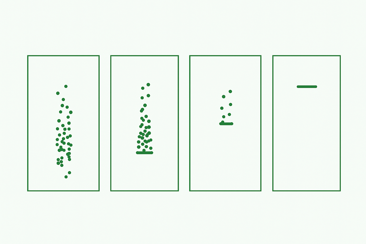
To assess the performance of the censoring method, we performed a similar simulation study as for the replacement method: finding the average mean and median standard deviation of 100 datasets when they are censored according to ten LOQs ranging between two and four. Figure 3 shows examples of a dataset on which censoring has been applied for a range of LOQs. Censored points are represented as having been moved to the LOQ for these plots.

A key difference between the replacement and censoring methods is how the mean and standard deviation of the censored data is calculated. Since censoring is being applied, we cannot use standard methods. Instead, we must fit the data with a normal distribution and read off the mean and standard deviation from the fitted model. The fitting method uses a combination of algorithms to account for the censoring in the data, meaning it is significantly more complex than using the replacement method. Nevertheless, it can be implemented fairly easily using statistical libraries in languages such as R or Python.

The results of the simulations using the censoring method are shown in Figure 4.

As with the replacement method, we see the relationship between the percentage of censored observations and the LOQ follows a S-shaped curve. The behaviour of the other metrics is noticeably different, however.

The fitted mean remains closer to the simulated mean for a larger LOQ range using the censoring method compared to the replacement method. In the latter, we saw that the observed mean dropped to around 2.5 by the time the LOQ reached 3, and the observed mean decreased continuously as the percentage of replaced observations increased. By contrast, the fitted mean remained close to 3 for LOQs as high as 3.25 for the censoring method, which included censoring percentages as high as 90%. After this point, the fitted mean increases away from 3 – this is a result of there being very few observations which are not censored to the LOQ, which continues to increase.

We see a similar improvement in performance of the censoring method compared to the replacement method when we look at the fitted standard deviation. Using the replacement method, the bifurcation of the observations led to the observed standard deviation to move noticeably away from the simulated standard deviation of 0.25. As with the mean, the model fitting algorithm of the censoring method results in a far more consistent output, with the fitted standard deviation remaining close to 0.25 until approximately 90% of observations were censored. After this point, with very few uncensored observations, the standard deviation decreases towards zero.

The censoring method, therefore, appears to perform noticeably better against out performance metrics than the replacement method. While fitting a normal model to the censored data is computationally more complex than the replacement method, it ensures that the resulting mean and standard deviation are closer to a true reflection of reality than when using the replacement method. The replacement method introduces biases even when only a small number of observations fall outside of an LOQ. By contrast, the censoring method does not introduce biases even when a large proportion of observations are censored.

Further, the replacement method is incapable of providing an accurate estimate of the variability of the observations when observations are replaced. Thanks to the model fitting inherent to the censoring method, we can ascertain the variability of the observations with good accuracy even when a majority of observations are censored.

As demonstrated the simulation results, both methods break down when too many of the available observations fall outside the LOQ. In the extreme case where all the data is outside the LOQ, then there is little we can do with either method to recover meaningful results. Applying the replacement method naively, we would find that the mean is \frac{\text{LOQ}}{2}$ and the standard deviation is zero. Similarly, the model fitting of the censoring method – when it converges – provides the mean as the LOQ and the standard deviation as zero. This doesn’t give us much useful information about our data and is likely to lead us to incorrect conclusions.

In such a situation, it may be worth taking a pragmatic view. What is it that you’re trying to show in your experiment? Say you’re measuring the concentration of some impurity in your product, and all the data from a certain batch falls below the LOQ of your analysis method. One can draw the conclusion that the concentration of the impurity in question must be so low that it can’t be reliably quantified, and thus the batch can be passed for release. That assumes that the acceptance criterion is sufficiently high that it doesn’t itself fall below the LOQ of the analysis method.

In rare cases, one might find themselves in a situation where even this pragmatic approach fails. Perhaps you’re transferring the analysis method to a new site, and the receiving unit does not have equipment with the same sensitivity as that in the sending unit. You might find that samples which were quantifiable at the sending unit fall below the LOQ at the receiving unit. This could result in datasets where none of the observations are quantifiable. Unfortunately, statistics can only get you so far in this scenario: if such a transfer is deemed essential, then a reassessment of acceptance criteria or an upgrade of equipment might be appropriate. Ultimately, involving a statistician early in the assay development process can help you maximise the decision-making information available from your data, even when LOQs prove problematic.