
How to Fit a 4PL Model
When we calculate a relative potency, we find the shift between the dose-response data from two samples. This is usually done by performing a calculation using the parameters from statistical models fit to the dose-response datasets. Clearly, therefore, we must estimate the model which best fits the data. This is a process which is – thankfully – outsourced to a statistical software package in most cases, so many bioassay scientists might not ever consider the methods behind fitting the models they are using for their assays. That’s where we come in: here, we will explore why we need statistical models in the first place, the mathematical procedure used to fit them to bioassay data, as well as some of the common fitting problems which can arise.
Statistical Models for Bioassay Data
We’ve discussed several models which are used for calculating relative potency, including the linear, 4PL and 5PL models. But why are these the models which we are regularly used?
Key Takeaways
- Accurate relative potency estimation depends on an appropriate statistical model. The article explains why the four-parameter logistic (4PL) model is widely used for bioassay dose–response data, and why it provides a better balance between flexibility and generalisation than overfitted models.
- Model fitting is an iterative optimisation process. The blog describes how a 4PL model is fitted by minimising the Residual Sum of Squares (RSS), introducing concepts such as residuals, parameter estimation and optimisation to show how software arrives at the best-fitting model.
- Understanding model fitting helps identify unreliable results. By explaining common fitting problems such as singular model fits and insufficient data, the article highlights why analysts should understand the fitting process rather than treating statistical software as a complete “black box”.
No discussion of statistical models can be without British statistician George Box’s famous quote “All models are wrong, but some are useful”. In essence, this statement highlights that no model can ever encapsulate reality in full detail. We are always abstracting away some degree of complexity in order for the model to be useable.
As we’ve discussed several times previously, bioassay response data typically forms an S-shaped curve. We expect to see flat asymptotes at high and low doses, with a steep linear region between them. We may not always see the whole curve in assay results – indeed, we often choose our dose range to limit the responses to the central linear portion. To calculate relative potency, we are interested in the overall shape and location of the data because the relative potency is encoded in the horizontal shift between the two curves. That’s where our statistical model comes in: the shape and location of the data is encoded in our model in a way which makes it easy for us to calculate the horizontal shift.
But, our model will always be a simplification of reality, While our response data will broadly form the expected S-shaped curve, this will not be perfect. We always expect there to be some variability: some responses might be slightly higher than expected, and some slightly lower. If we were interested in reflecting this variability for a single dataset, we could choose a model which effectively “joins the dots”, with all the variation we observe encoded directly into the model parameters. An example of a model which does this is shown below. The model here is a 7th degree polynomial which has enough flexibility to pass every point exactly, meaning it captures the variation of this dataset exactly.
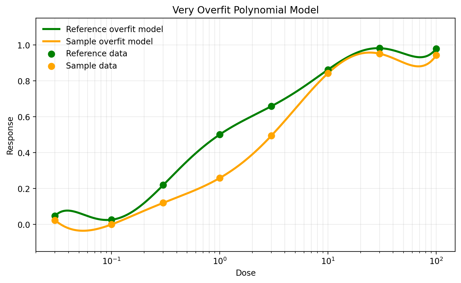
But this does not serve our purpose of modelling bioassay data to calculate relative potency. We want a class of model which can represent a range of possible datasets which could be generated by the assay. This polynomial model represents this specific dataset very well, but it is so specific to the shape of the data that it is unlikely that a future dataset would have a similar shape. We call such models overfit: they are a good representation of only a small subset of the possible datasets which are likely to be encountered.
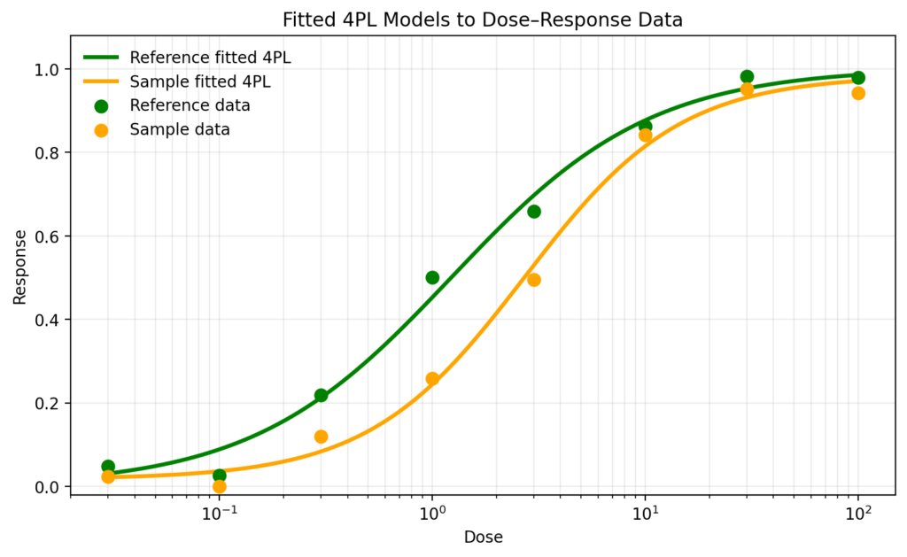
A model such as a 4PL is far more useful in this scenario. While it is a superficially simpler model which encodes less information about a single dataset, it gives a good representation of the typical dose-response relationship for the assay. The plot below shows the same data fitted using 4PLs. Using these models, we can make a good estimate of the horizontal shift between the two curves, and, therefore, the relative potency.
Model Parameters
We often think of statistical models in terms of how we have displayed them here: a curve on a graph. While this representation is a critical visualisation tool for getting a feel for the model, we use a different approach when it is being fit. Specifically, we must represent the model in terms of its parameters. A statistical model is uniquely defined by its parameters, and it’s their value which determines the shape we observe when we plot the model. The parameters are used in the mathematical formula, or parameterisation, which describes the model.
You can think of a parameterisation like a synthesiser. We input a dose, which is like pressing a key on the keyboard, and we get a response out, which is like the note we hear. The parameters, then, are the dials on the synth: their specific positions define how the produced note sounds to a listener. In the same way, the specific values of the parameters determine the relationship between each dose and response, and, therefore, the shape of the model we observe when plotted.
Here, we’re going to be focussing on the four-parameter logistic model, or 4PL. We’ve gone into great detail about this model in the past, but we will give a short overview here. As we would expect from the name, a 4PL model requires four parameters, often labelled A-D. These are:
| Parameter | Role |
|---|---|
| A | Zero-dose asymptote |
| B | Slope parameter |
| C | EC50 |
| D | Infinite-dose asymptote |
These combine in the parameterisation below, where the response is \(y\) and the dose is \(x\):
\[y=D+\frac{A-D}{1+e^{B\left(\log x-\log C\right)}}\]Fitting a 4PL Model
So, given a set of data, how do we go about fitting a 4PL model? We need an approach which quantifies how well a model fits a set of data. One such method uses the Residual Sum of Squares, or RSS.
The first step is to make a guess at some parameter values, which defines an initial model. A possible set of initial choices for the parameters could be to set:
- A to the lowest response
- B to 1
- C to the middle dose of the series
- D to the highest response
We then calculate the residuals from the data to the initial guess. The residual is the difference between the observed response and the response predicted by the model for a particular dose. That is:
Where \(x_i\) is the dose, \(y_i\) is the observed response in the dataset, and \(\hat{y}\) is the predicted response from the model. We calculate the residual for each observation in the dataset, square them, and add them together to give the Residual Sum of Squares (RSS). The RSS is defined mathematically as:
\[RSS=\sum_i r_i^2\]The RSS gives a measure of the distance of the initial model to the observed data. We want our model to be as close to the observed data as possible, so we want to minimise the RSS. Therefore, once we have calculated the RSS for the initial guess, we update our choice of model parameters to a new set of values. We once again assess the RSS, and if it is lower, the model with those parameter values is an improvement. We then repeat this process until no new set of parameters can be found which further reduces the RSS.
Why do we square the residuals? There are several reasons. One relates to maximum likelihood theory, which we will not explore here, and another is that the maths turns out to be simpler when working with squared residuals. A consequence of this is that it penalises large residuals more than small residuals.
For simple cases, such as linear models, the optimal model can be found analytically, but this is not possible for complex models such as the 4PL. That means we must perform an iterative process to fit the 4PL. As a result, we run into the question of efficiency: how can we find the best fit model in the fewest steps possible?
One such approach is known as gradient descent optimisation. Intuitively, this method is like navigating down a mountain in a thick fog. If you can’t see what direction you need to go, you might take a step in each direction until you find one which takes you downhill. Once you’ve found that, you take a step in that direction, and repeat the process.
The gradient of a function, represented by \(\nabla\), is its slope in multidimensional space: it tells us how quickly and in which direction the function changes as its variables change. Taking the gradient is like finding “down” in the foggy hill scenario: it finds the direction in which the parameters should be changed to reduce the RSS further. In our case, we’re interested in how the RSS of our model changes when you vary the model parameters. There will be a component of the gradient for each of our four parameters, which correspond to how the RSS changes with that parameter assuming the other three parameters are kept constant.
To update the parameters for a new iteration of the algorithm, we use the gradient component for each parameter according to:
\begin{align} A_{New}&=A_{Old}-L\nabla_A\\ B_{New}&=B_{Old}-L\nabla_B\\ C_{New}&=C_{Old}-L\nabla_C\\ D_{New}&=D_{Old}-L\nabla_D \end{align}Where \(\nabla_A\) is the gradient component of the RSS for the A parameter, \(\nabla_B\) is the gradient component of the RSS for the B parameter, etc. \(L\) is the learning rate: it defines the amount the parameters change on each step of the iteration – the size of the step down the hill. If the learning rate is too small, the algorithm will be too slow to converge on the optimal solution, while if it is too large, the optimal solution might be missed.
Let’s examine how this method pulls the A parameter in a direction which reduces the RSS. For now, we’ll assume \(L=1\). If \(\nabla_A\) is positive, it means that the RSS increases as A increases. So, subtracting \(\nabla_A\) means that \(A_{New}<A_{Old}\), so the RSS will be smaller with \(A_{New}\) than with \(A_{Old}\).
Conversely, if \(\nabla_A\) is negative, it means that the RSS decreases as A increases. Subtracting the negative \(\nabla_A\) means that \(A_{New}>A_{Old}\), so the RSS will be smaller with \(A_{New}\) than with \(A_{Old}\).
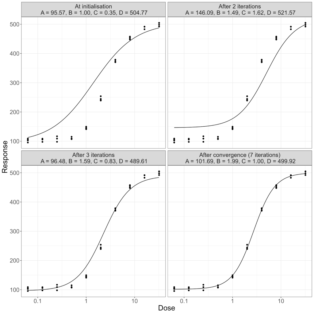
The figure below shows an example of a model fitting algorithm in action. We see the fitted curve and model parameters at a series of steps during the fitting process. Notice how the initial guess is quickly improved by the algorithm, which reaches an optimal model after just seven iterations.
Common Model Fitting Errors
No algorithm is perfect, and the model fitting process we’ve describe here is no different. Any failure is frustrating, and it can be made even more so by opaque error messages in some statistical software packages commonly used to fit statistical models.
A singular model fit is one where the algorithm does not have sufficient information to reliably determine one or more of the model parameters. Why singular? In practice, model fitting in most software packages relies on solving a system of equations – four, in the case of the 4PL – using matrices. If, for some reason, the matrix cannot be inverted then the equations cannot be reliably solved. We call such a matrix singular, and so the model is singular too.
One common way for a singular model to occur is when changing either of two parameters has more or less the same effect on the model. For example, if all the observations sat on the lower asymptote – if our dose range was too low to elicit a response, say – then it would be impossible to distinguish between the effect of B or C parameter changes on the model fit as we do not observe a linear region in the data. That means there are a large (or even infinite) number of possible models which fit the data equally well. In such cases, many software packages will, in essence, take a guess at the parameters and report an extremely wide confidence interval. If your software doesn’t have a check for singular model fits, then it is important to keep an eye on your results for these expansive confidence intervals as the parameter values produced from such model fits cannot be relied upon.
Other scenarios which can generate singular model fits for a 4PL include datasets which are limited to only the linear region. This is almost the inverse of the example we discussed previously: the model fitting algorithm can easily determine the B and C parameters, but it does not have sufficient information to reliably determine either asymptote from the data. Additionally, singular fits are expected to occur when there is insufficient data to fit a 4PL. To fit any model with parameters, one must have at a minimum the same number of observations. So, for a 4PL, we require a minimum of 4 observations: fewer will leave the fitting algorithm unable to reliably determine the optimal parameters. In some cases, a zero-dose control sample can be used as an additional data point to allow a 4PL to be fit if only four observations are available.
A Critical Black Box?
In most cases, statistical model fitting is a push of the enter button or a click of the mouse. It is the process which occurs behind the scenes while an analyst grabs a quick cup of coffee. But, while it may not be a hands-on process, ensuring it performs well is still a critical component of the bioassay analysis process. As we have seen, a well-fit model of the right type is vital for a good estimate of the relative potency of a sample, and it is all too easy for the process to go wrong if there are issues with collected data. When model fitting failures occur, some software packages spit out potentially misleading results which, if used blindly, could lead to incorrect decisions being made about product quality. Others, including QuBAS, flag the analysis as a failure, providing an important fail-safe to prevent spurious data moving down the pipeline. Regardless, it is essential to have an understanding of the model fitting process for your assay so that any problems can be easily resolved.