
Defining Precision: Variance Components Analysis for Bioassay
A bioassay result is never certain. We are never able to measure the relative potency of a product, say, with 100% confidence that our answer is “correct”. There will always be an amount of variability in our measurements, due to both the assay condition and procedure. This is why results are typically presented with a confidence interval – this represents the plausible range in which the “correct” answer is expected to fall and reflects the variability of the assay.
As a result, it is crucial to have a good understanding of the variability of an assay procedure. This information can be used to inform replication strategies alongside other optimisations to maximise the precision of the assay. Here, we’ll discuss the statistics that goes into understanding the assay variability – the Variance Components Analysis – and how it provides a breakdown of the factors that influence the variability of a bioassay.
Key Takeaways
- Variance Components Analysis (VCA) quantifies assay variability. By partitioning total variance into individual sources, VCA helps scientists understand which factors contribute most to variability in bioassay results.
- Different sources of variability affect assay precision differently. Factors such as analysts, reagent lots, cell aliquots, runs, and plates can each contribute to overall assay variability, with some sources having a much greater impact than others.
- VCA supports informed assay optimisation. By identifying the largest contributors to variability, laboratories can focus improvement efforts where they will have the greatest effect on assay precision, robustness, and validation performance.
Precision and Variability
The precision of an experiment relates to the spread of results over a repeated series of measurements. The closer the results are to each other, the more precise the experiment is. The spread of the results is known as the variability of the experiment. Variability is often quantified by the standard deviation – representing the typical difference between the observations in a dataset and the mean of those observations – but it is often easier mathematically to work with the variance, which is the square of the standard deviation.
There are several aspects of precision we can investigate for an experiment. These represent the variability of the experiment under different conditions. The most fundamental level of variability is repeatability, which is the variability between experiments performed when the conditions are kept as similar as possible. This represents the underlying variability of the experiments before any other factors are included.
Add back in some of those factors and we have the intermediate precision. This is the variability of the experiment under normal laboratory operating conditions, e.g. with different operators and reagent lots, and between different days. The intermediate precision is an important property of a bioassay to understand as it is the most representative of the variability in day-to-day use.
Variance Components
In theory, any aspect of a bioassay procedure could result in variability. Factors as simple as different reagent lots or as outlandish as seasonal variations in sunlight can cause variability in the results of an assay. Nevertheless, there are some factors which can be easily investigated in a variance components analysis.
Inter- and Intra-Run Variance
Many assay analysis procedures include several runs, which themselves consist of several plates. A plate is, as it sounds, a single bioassay plate. A plate may contain several samples, but it is typically the case that a plate provides a single result per sample. A run, then, combines the results across several plates to give a single, collective result. An additional layer of replication can be added by combining the results from multiple runs, if required. The format of the procedure is the specific combination of runs and plates used for a procedure.
Most assay procedures can benefit from assessment of variance within and between runs. Within-run, or intra-run, variance is that which occurs between the plates which make up a run. The between-run, or inter-run, variance is that which occurs between the runs which make up an assay procedure. The plot below shows an example of data from an assay with two plates per run.
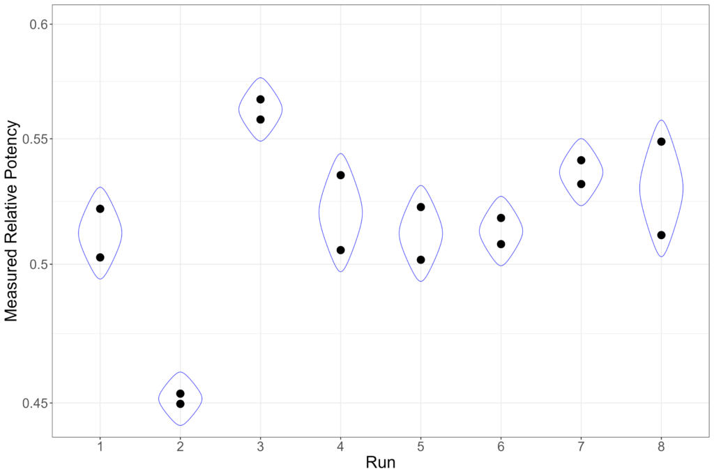
The measured relative potency from each plate is shown. The intra-run variance is the variability between the measured relative potency values from each run.
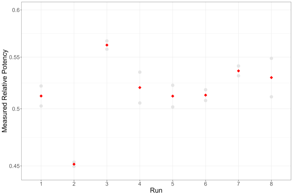
The variability of the combined potency values is then the inter-run variation. This is shown in the plot above. We can see that, for this procedure, the inter-run variance is greater than the intra-run variance. This is the more common arrangement: the plates within a run are more likely to experience similar conditions than those in different runs, which leads to smaller variability.
Conditional and Procedural Components
A focus on the inter- and intra-run variance is helpful for understanding where in the assay process variability arises, but it doesn’t tell us much about the source of that variance. Which aspects of the procedure introduce the most variance? This is the question which a variance component analysis seeks to answer.
For example, analyst variance is one which is commonly investigated. Different analysts might have minor differences in pipetting technique, timing, or interpretation of the procedure, all of which can introduce variability. Reagent lots are also a factor which can be considered in a variance components analysis. Assays typically require a number of reagents and other materials to enable the reaction with the product in question. These will be manufactured to a very high standard and consistency, but there will inevitably be differences in the reaction between reagent lots.
Constructing a Variance Components Analysis
Imagine now that we want to perform a variance components analysis for a certain procedure. We’ll assume that the procedure format consists of one run of two plates. The procedure will be run every day, and will utilise multiple analysts and reagent lots. How do we set up the analysis?
A VCA often utilises a mixed effects model. In statistics, variance factors can fall into two categories, fixed or random. Fixed effects are those whose levels are of direct interest. For a bioassay, this often includes nominal potency level of the sample: we are specifically interested in the measured relative potency for, say, a 100% potent sample.
Random effects, on the other hand, are factors for which their specific levels are not relevant. Instead, the levels of such factors are treated as a random sample of all possible levels. The analyst, for example, is often treated as a random effect. Whether the analyst is Alice, Bob, or Caroline isn’t strictly relevant, all we are interested in is the amount of variation that factor introduces into the results. For our scenario, the analyst, day, and reagent lot are treated as random effects.
When considering random effects, we must be careful to account for any interactions between the effects. There are three main ways this can happen:
Nested Factors: A factor is nested with a second factor when each level of that factor only occurs in conjunction with a single level of the second. A common example in bioassay might be the structure of plates and runs. Let’s imagine we designate runs numerically (Run 1, Run 2, etc) and plates alphabetically (Plate A, Plate B, etc) – this labelling highlights that plates in different runs should not be considered as the same. Run 1 might consist of Plates A and B, Run 2 has Plates C and D, and so on. We then say that the plates factor is nested with the runs factor: Plate A only occurs in Run 1; Plate C only occurs in Run 2. This can be further extended to include procedures and days: indeed, it is common for plates, runs, procedures, and days to be treated as nested factors.
When dealing with nested factors, it is important to account for the variance from factors higher up the nesting ladder. If plates are nested with runs, then the plate-to-plate variance must be calculated after accounting for the run-to-run variance, for example.
Crossed Factors: Two factors are crossed when every level of a factor occurs with every level of another. So, the analyst factor might be crossed with the day factor if every analyst performs one run within the procedure on every day. This structure allows the effects due to the two crossed factors to be easily separated. Say the measured relative potency is unusually high on a certain day. Since each analyst performed a run that day, it is easy to distinguish whether the unusual result can be explained by an analyst effect or whether there was some condition in the lab that day which caused the results from all analysts to be higher than usual.
Confounded Factors: Two factors are confounded when the effects from one cannot be distinguished from another. For example, the analyst factor might be confounded with the reagent lot factor if each analyst only uses a single reagent lot for their analyses. This means that we cannot tell whether the variance in the results is due to analyst effects or reagent lot effects.
For our example, we’re going to follow the example data provided in Appendix B of the latest draft of USP <1033>. This investigates 3 factors: the Analyst, the Media lot, and the Cell Aliquot. Each factor has two levels, and is crossed with the other two. This means that across 8 procedures, all levels of the three factors occur with each other at least once, as shown in the table below.
| Procedure | Analyst | Media Lot | Cell Aliquot |
|---|---|---|---|
| 1 | 1 | 1 | 1 |
| 2 | 1 | 1 | 2 |
| 3 | 2 | 1 | 1 |
| 4 | 2 | 1 | 2 |
| 5 | 1 | 2 | 1 |
| 6 | 1 | 2 | 2 |
| 7 | 2 | 2 | 1 |
| 8 | 2 | 2 | 2 |
Having determined the factors of interest and the relationships between them, we can proceed with fitting the mixed effects model. This can be written as:
\[y_{ijkl}=\mu+F_i+A_j+M_k+C_l+\epsilon_{ijkl}\]
This may seem complicated, but each term corresponds to one of the factors which contribute the variance of the measured relative potency. The table below lists their meanings:
| Term | Meaning |
|---|---|
| \(y_{ijkl}\) | A relative potency observation |
| \(\mu\) | The grand (overall) mean |
| \(F_i\) | The fixed effect for potency level i |
| \(A_j\) | The random effect for analyst j |
| \(M_k\) | The random effect for media lot k |
| \(C_l\) | The random effect for cell aliquot l |
| \(\epsilon_{ijkl}\) | The residual variance (random error) |
The index i, indexes the tested potency levels (50%, 71%, 100%, 141% and 200%), while the indices (j, k, l) specify the level of each factor: 1 or 2. The residual variance is whatever variance is left over after all the other factors are accounted for.
We won’t go into the details of how the model is fitted, but, in short, we assume each of the random effects follow a normal distribution centred on zero with an unknown variance. The value of those unknown variances is the goal of the exercise: they tell us how much variability we can expect the random effects to contribute.
Applying a VCA to the data, our results look like this:
| Component | Variance Component | % Total Variance |
|---|---|---|
| Total | 0.0065 | 100% |
| Analyst | 0.0020 | 31.3% |
| Media Lot | 0 | 0% |
| Cell Aliquot | 0.0017 | 26.5% |
| Residual | 0.0027 | 42.2% |
From the analysis, we can see that the biggest influence on the variability of the assay is the residual variance – plate-level variance from, for example, plate effects. The analyst and cell aliquot have a smaller effect, but still carry a sizable proportion of the total variance. Conversely, there is no influence on the assay from the media lot, which indicates that the media lot does not contribute variability to the measured relative potency.
How do these variance components map back to the concepts of precision which we discussed earlier. Well, repeatability is how variable our result is when we keep everything as similar as possible, so we do not vary the analyst, media lot, or cell aliquot. That means the repeatability is just the residual variance.
The intermediate precision, on the other hand, represents the variability under normal running conditions of the assay, which includes changes in the factors we’ve investigated. This is the measure of precision which is typically used when evaluating the performance of the assay in, for example, a validation exercise. We, therefore, add the components for the analyst and reagent lot back in and find:
\[\sigma_{IP}^{2}=\sigma_A^{2}+\sigma_M^{2}+\sigma_C^{2}+\sigma_{\epsilon}^{2}=0.0065\]In this case, the total variance is indeed the intermediate precision, which corresponds to a %GCV of 8.4%.
A variance components analysis allows for an in-depth assessment of the factors which contribute to the variability of an assay. This means that the assay procedure can be optimised to improve its precision. In our example, the VCA highlights that the analyst accounts for 30% of the total variability. Perhaps further training for the analysts conducting the assay might be an easy way to improve its precision should it be required. Conversely, there would be little point in imposing stricter controls on the media lots since there is no evidence of these contributing to the variability of the assay. These decisions are made possible by using a VCA to assess the factors which affect the variability of the assay results and understanding their contributions to the total variance. The VCA is, therefore, a simple but powerful procedure which forms a critical lynchpin in the bioassay lifecycle.