Matching Adjusted Indirect Comparison (MAIC) – 4 Practical steps to follow
When comparing trial outcomes using standard network meta-analysis (NMA), the assumption is that populations in different trials do not differ in any characteristics that may impact the treatment effect (see this blog for an introduction to the concept of NMA). If this assumption is not true, these study differences then need to be accounted for when comparing treatments.
In an earlier blog, we have introduced the concept of population adjustment to account for differences between trials that may have an impact on the absolute outcome (prognostic variables), or relative treatment effect (effect modifying variables) when doing a network meta analysis or other indirect treatment comparison.
In this blog, we will introduce the following steps required to conduct a MAIC (Matching Adjusted Indirect Comparison):
- Step 1: Compare the characteristics of the trial to be weighted against the target population
- Step 2: Calculate and check the MAIC weights
- Step 3: Check the balance of the weighted trials
- Step 4: Compare the weighted and the unweighted outcome, and evaluate the uncertainty
We demonstrate these steps using a simple example where we have two trials, A and B, with individual patient data (IPD), and a target population C where only summary data is available.
Key Takeaways
- MAIC is used to adjust for differences in baseline characteristics between trials when only one trial has individual patient data and the comparator has only summary data.
- Before weighting, you must compare study populations and select prognostic and effect-modifying variables that are available in both the IPD trial and the target population.
- Calculated MAIC weights need careful checking; extreme or near-zero weights can indicate poor overlap between studies and greatly increase uncertainty.
- After weighting, confirm that the adjusted IPD trial actually matches the target population on key covariates (e.g. means, proportions).
- Weighting reduces the effective sample size and widens confidence intervals, so conclusions about treatment differences must be made cautiously.
- Conducting a MAIC is often iterative: you may need to revisit which variables to include and repeat the process if diagnostics look poor.
Unanchored comparison between the single arm trials A and C and between B and C
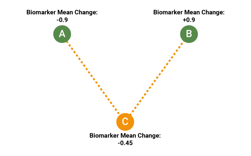
All three trials have 50 participants. In each trial, a different treatment has been evaluated with the purpose of keeping the value of a biomarker as low as possible. In Trial A, the observed change was -0.9 (standard error 0.17); in Trial B, the observed change was +0.9 (standard error 0.15); in Trial C, the observed change was +2.0 (standard error 0.15). The standard error of the change was approximately 0.15 in all three trials. In this example, all three trials are single-arm trials, so we can’t create a network, and will therefore have to conduct an “unanchored” MAIC, comparing the treatment arms directly.
When conducting a MAIC, the focus is on the participants and how they differ between the trials of interest. When conducting population adjustment, we assume that there is individual patient data available for a Trial A, and summary data available for a target population, usually the study population of another Trial C. Using MAIC, we can then give weights to the participants of A so that the new, weighted population demographics are as similar as possible to the summary data of C.
Step 1: Compare the characteristics of the trial to be weighted against the target population
Since we are conducting an unanchored MAIC, we will need to adjust for both potential effect modifiers, and for potential prognostic variables (see our previous blog for details).
The figure below illustrates the distributions of the variables of two Trials A and B where we have individual patient data (IPD), compared with the reported average in a Trial C where we only have summary data. In our example, we assume that these are all the variables that are reported in both A/B and in C – in an unanchored MAIC, one usually starts by considering all available variables.
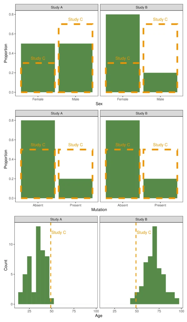
The dotted orange line shows the distribution from Trial C overlaid on the distributions from Trials A and B in green.
From the figure, we can see that Trial A has a younger population with a more even gender distribution and lower mutation rates than Trial C. We can also see that Trial B has a largely female, older population, again with a lower mutation rate. All of these different characteristics may affect the success rate of a treatment (or affect any other outcome of interest). In addition, one or more may be a treatment effect modifier, such that one treatment may be expected to perform better than another.
Exploring the trials in this way gives us an idea of what characteristics might be important to adjust for. For example, the difference in mutation rate seems likely to be important; the age distribution of Trial B also stands out as it is much higher than in C, with no patient below the average age of C.
Step 2: Calculate and check the MAIC weights
Once we have chosen the variables to adjust for, the weights can be calculated. For a given variable, the MAIC is designed to give those participants that are most similar to the average in the target population a high weight, and those that are unlike the target population a low weight. We will not go into the mathematical details of how to calculate the MAIC weights in this blog; NICE provides detailed instruction and R code – http://nicedsu.org.uk/technical-support-documents/population-adjusted-indirect-comparisons-maic-and-stc/
There is also a recently released R package that looks promising – (however, we have not evaluated this, so can make no guarantees as to its reliability) https://cran.r-project.org/web/packages/maic/index.html.
Regardless of how you calculate the weights, the result of the procedure needs to be checked. The following figure shows how the calculated weights are distributed for Trial A and Trial B, respectively.
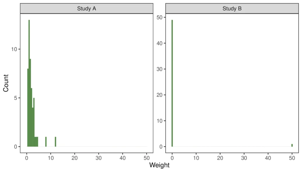
It is important to evaluate the distribution of weights. If there are too many participants being allocated near-zero weights, that is indicative of the trials being quite different and may increase the uncertainty of the results. Similarly, if a small number of participants are given very high weights, these participants can skew the results.
From the figure, we can see that Trial A has a reasonably high proportion of participants with low weights and a smaller number of patients with high weights. Ideally, the weights would be more evenly distributed around 1, but what is seen is not uncommon when the IPD trial population is somewhat dissimilar from the target population.
The weight distribution of Trial B is an example where the matching process goes wrong. In this case, one participant has been given a weight of 50, while all other patients have been given a weight of zero.
Step 3: Check the balance of the weighted trials
The two tables below show how the distribution of variables change when calculating weighted averages using the weights from Step 2.
For Trial A, the weighting procedure has successfully adjusted the distributions of variables to match those reported for Trial C. Thus, we can expect that the effect of these variables on the biomarker change is minimised when using a weighted analysis.
However, for Trial B, it is clear that something has gone wrong – the weighted distribution of variables is quite dissimilar to the distribution in C. This MAIC was therefore unsuccessful, and the weights are unsuitable for further analysis. On closer inspection, it is clear what has happened; the youngest participant in the trial was 48 years old, so the MAIC procedure selected this participant to minimise the difference from C, giving all other participants a weight of 0.
In more complex settings, the reason for the MAIC weighting process to fail may not be so obvious, but always indicates that the two trials are very dissimilar with respect to the included variables. A close inspection of the study population and/or dropping some of the variables may help to resolve the issue.
Table 1: Weighting of Trial A
| Variable | Original distribution in A | Weighted average | Reported distribution in C |
|---|---|---|---|
| Age (years) | 34.74 | 45 | 45 |
| Female proportion | 0.54 | 0.25 | 0.25 |
| Male proportion | 0.46 | 0.75 | 0.75 |
| Mutation – Absent | 0.84 | 0.50 | 0.50 |
| Mutation – Present | 0.16 | 0.50 | 0.50 |
Table 2: Weighting of Trial B
| Variable | Original distribution in B | Weighted distribution | Reported distribution in C |
|---|---|---|---|
| Age (years) | 68 | 48 | 45 |
| Female proportion | 0.76 | 1 | 0.25 |
| Male proportion | 0.24 | 0 | 0.75 |
| Mutation – Absent | 0.84 | 1 | 0.50 |
| Mutation – Present | 0.16 | 0 | 0.50 |
Step 4: Compare the weighted and the unweighted outcome, and evaluate the uncertainty
The final step is to calculate the weighted outcome. This can be done using a simple weighted average of the outcome in Trial A, or using a weighted linear regression without covariates. The advantage with the latter approach is that you can then make use of so-called “sandwich” estimators for the variance, which will give you correct confidence intervals, accounting for the fact that the weights themselves have been estimated. An additional way to evaluate the uncertainty of the fit is by calculating the effective sample size, using the equation \(\mathrm{ESS} = (\Sigma w)^2 / \Sigma(w^2)\), where \(w\) refers to the weights.
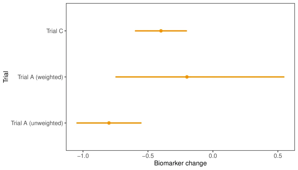
In the figure above, we can compare the weighted and unweighted estimate for mean biomarker change in Trial A to that in Trial C. The weighted Trial A result has shifted closer to Trial C; however, the 95% confidence interval has increased drastically. This is also reflected in that the ESS for the A MAIC was five, ten times smaller than the study size of 50. Thus, while the point estimate indicates that the difference between A and C might be smaller when accounting for differences in age, sex, and mutation, the uncertainty introduced by the weighting procedure means that we have to be very careful when drawing conclusions from the results.
Summary
To recap, when conducting a MAIC, there are four steps to keep in mind:
- Check the original study characteristics.
- Check the calculated weights.
- Check that the weights reduce study differences.
- Check the level of uncertainty of your weighted analysis.
This often becomes an iterative process – if any of the steps indicate a cause for concern, it may be worth revisiting the study characteristics, and possibly conducting another MAIC with a subset of the variables included.
For further reading, the NICE technical support document 18 has an in-depth explanation (http://nicedsu.org.uk/technical-support-documents/population-adjusted-indirect-comparisons-maic-and-stc/), as does the accompanying paper (https://pubmed.ncbi.nlm.nih.gov/28823204/).