Complications of fitting 4PL and 5PL models to bioassay data
We have previously discussed the 4 parameter logistic (4PL) model. Sometimes you may see slightly different versions of the 4PL equation – these are all mathematically equivalent. However, one thing to watch out for is that the meanings of the four parameters can vary between these versions. If you’re fitting a 4PL and getting parameter values very different from those you were expecting, check that you’re using the version of the 4PL you thought you were! We examine this in more detail in this blog about the 4PL formula.
Here, we’ll go into more detail about models for continuous response data, and in particular some of the problems that can arise.
The 4PL is a symmetrical curve, which starts out at an asymptote (a constant value) at low doses, increases in an S-shaped curve, and ends up at another asymptote at high doses.
Key Takeaways
- The 4-parameter logistic (4PL) model is symmetrical and works well for many bioassays, but it struggles with asymmetric data; the 5-parameter logistic (5PL) adds an extra parameter (E) to account for asymmetry.
- Least squares fitting can still produce poor fits if the model doesn’t match the data; a 4PL can fail for asymmetric data and even a 5PL can be inadequate if the asymmetry is extreme.
- Goodness-of-fit tests and warning signs (e.g., very large slope values or failure to converge) help detect issues; adjusting dose spacing or using software with built-in checks can help avoid misleading results.
An example 4PL curve for bioassay data is shown in the figure below. A and D are the asymptotes, and the EC50 is antilog(C). B is the “slope parameter”, which is proportional to the slope.
The equation for the 4PL model takes the form
\[y=D+\frac{A-D}{1+e^{B\left(\log(dose)-C\right)}}\]
for a response y and raw dose x.

The 5 parameter logistic
The 4PL often fits bioassay data quite well. But since it is symmetrical, it will not fit asymmetrical data well. In this case a commonly-used alternative is the 5 parameter logistic (5PL) model. This is similar to the 4PL but has an additional parameter, E, which allows it to be asymmetric. The equation for the 5PL, again for response y, is:
\[y=D+\frac{A-D}{\left[1+e^{B\left(\log(dose)-C\right)}\right]^E}\]
Like the 4PL, the 5PL starts at one asymptote at low doses and ends at another asymptote at high doses. However, the curve from one asymptote to the other is not symmetrical.
The asymptotes are A and D again, while B is again the slope parameter. However, the EC50 is not antilog(C) for the 5PL. Instead, it is given by:
\[EC_{50}=C+\frac{1}{B}\ln(2^{\frac{1}{E}}-1)\]

The new parameter E controls the asymmetry: if E is 1 the curve is symmetric. For larger values the part of the curve near the A asymptote becomes more tightly curved while the part near the D asymptote is less curved; for values below 1 it is the other way around.
The fitting process
To understand some of the problems that can arise when using the 4PL and 5PL, it is important to have an idea of what bioassay statistical software does when it “fits” a model. Statistical software uses a method called “least squares” fitting. This method has the advantages that it is mathematically simple, and it is consistent with the assumption that the data follows a normal distribution.
Robust regression is an alternative approach to this but that will be discussed in a later blog.
Least squares fitting, as the name suggests, tries to minimise the sum of “squares” – that is, the squares of the distances between the data and the model curve. This makes sense because making these distances small will make the curve be close to the data, which is what we want.
It is impossible to directly calculate the best fit 4PL or 5PL model through a single equation. Instead, bioassay statistical software starts with a rough guess at the values of A, B, C and D (and E if 5PL), which may be quite far from the best fit. It then tries to adjust this fit a little and checks whether the sum of squares has decreased. If it has, it accepts the change and then tries another one; if not, it tries a different change to the curve. This continues until it is impossible to find a change that decreases the sum of squares, in which case the software concludes that it has found the best fit.
Problems with fitting
Normally the fitting process works well. However, in some situations it can give unexpected results.
One example is that the “best” fit determined by the software can still be very poor. This happens if we try to fit bioassay data to an inappropriate model. For example, if the data is asymmetric but we try to fit a 4PL, there is no way the fit can be close to the data everywhere, since the 4PL is inherently symmetric. Another example is if the bioassay data are extremely asymmetric and we try to fit a 5PL. Although the 5PL is asymmetric, there is a maximum amount of asymmetry possible. Figure 3 shows the full range of asymmetry possible for a 5PL model.

All the curves in this plot are 5PLs, with different values of the E parameter. The black curve is E=1 (symmetric), and the dotted curves are other values of E. However, it is impossible to go beyond the solid purple curve on the right side (E=0) or the solid red curve on the left (E=∞). So if your bioassay data is more asymmetric than this, it will be impossible to get a good fit with a 5PL.
An appropriate goodness-of-fit test, for example the F test, is useful to check whether this is happening. The F test can be used as a goodness-of-fit test for any model as long as there are two or more replicates. The F test compares the “lack-of-fit” error (how far the fit is from the bioassay data) and the “pure error” (how far apart the replicates are, on average). If the former is large compared to the latter, the p-value for the F test will be small, indicating a poor fit.
Another issue is that the fit can be close to the data, but the model curve may not be as expected. For the 4PL, we can end up with curves like Figure 4.
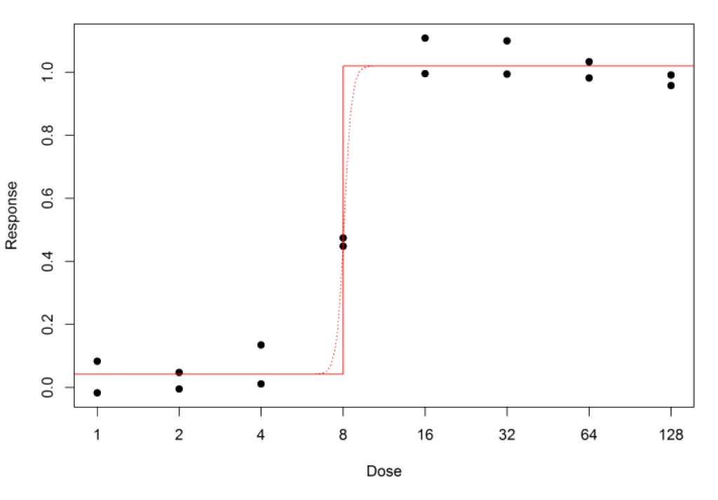
Well, with the bioassay data shown above it so happens that the sum of squares always becomes smaller if B is increased – but more and more gradually as B increases. Mathematically, the best fit has infinite B, which means the model curve is flat all the way up to the EC50, where it abruptly jumps to the other asymptote.
A particular problem with this situation is that it may not be as obvious as the example above that it is happening. Most bioassay statistical software will adjust the fit by increasing B a large number of times, but eventually the change in the sum of squares becomes so small that the software concludes that it has reached the best fit, and stops.
It will then output whatever value of B it has reached, which might be something like 10 or 20. This will give a steep model curve, without an abrupt jump. There may be no obvious sign anything is wrong.
To avoid this problem, always examine the software output for warning messages – in this situation, the output might say something like “Fit failed to converge” – and consider using suitability criteria which reject fits with very large values of B. If this happens repeatedly, it may be necessary to decrease the spacing between doses to get more data on the steep part of the curve.
Quantics’ bioassay software, QuBAS, deals with this problem automatically: it specifically checks whether what looks like the best fit is a sensible smooth curve.
Is the biological data presented above really always unexpected? This interesting paper by Greulich et al had us thinking here at Quantics.
A similar “jump” can also happen for 5PL fits. Our purple curve in the 5PL example shows a different case where the response is exactly flat up to a certain dose, where it suddenly starts going steeply upwards.
However, Greulich et al used a simple mathematical model for bacterial growth in the presence of antibiotics and found curves that look rather similar, using an equation very similar to the 5PL. The authors also find that their model fits experimental data quite well. So maybe these “unexpected” fits can happen after all?