Improving confidence limits for concentration-response models with quantal data

In ecotoxicology statistics there are three main types of data:

1. continuous
2. discrete
3. quantal / binary

Continuous data is that which can take a (numerical) value over a continuous range (e.g. weight), and discrete data is that which takes a finite number of values (e.g. colour). Quantal data is the focus of this blog post; it is data where the response can take only one of two values (e.g. mobile / immobile or alive / dead); it is often recorded as the number of affected individuals out of the total number of individuals in each experimental unit.

The previous post described the advantages of modelling the concentration-response relationship, and this post describes one possible (OECD-approved) approach to modelling this relationship

Read our NOEC and LOEC blog here

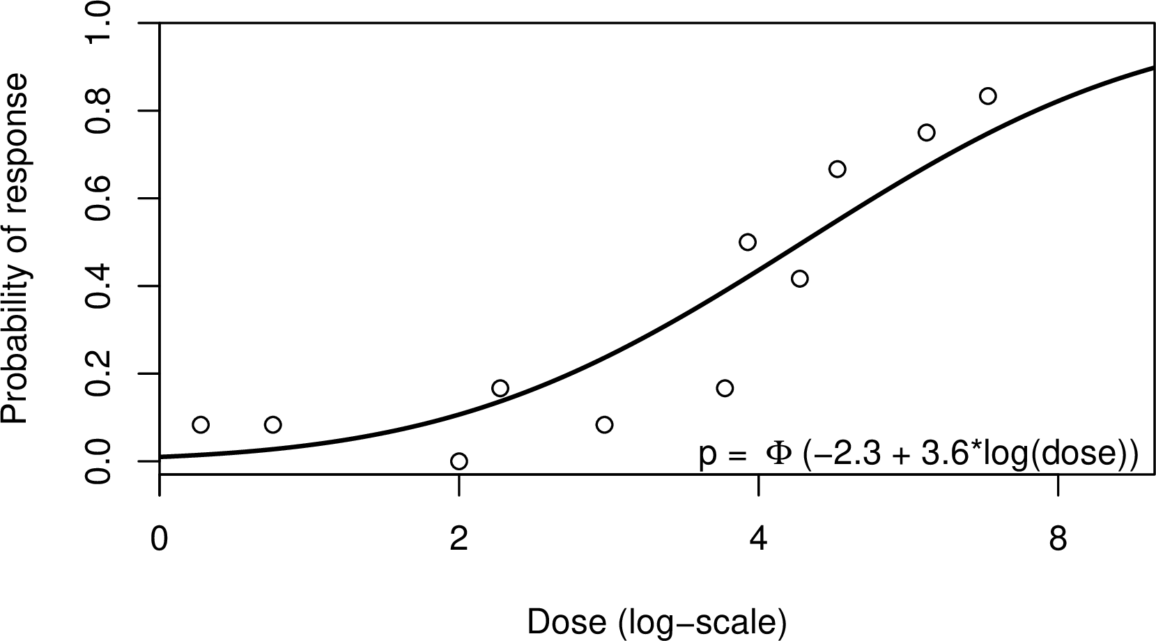
A popular choice for concentration-response modelling for quantal data in ecotoxicology is the probit model. This model is useful because it is restricted to returning values between 0 and 1 (or 0% and 100%), and it is monotone i.e. non-decreasing (or non-increasing, depending on the nature of the response).

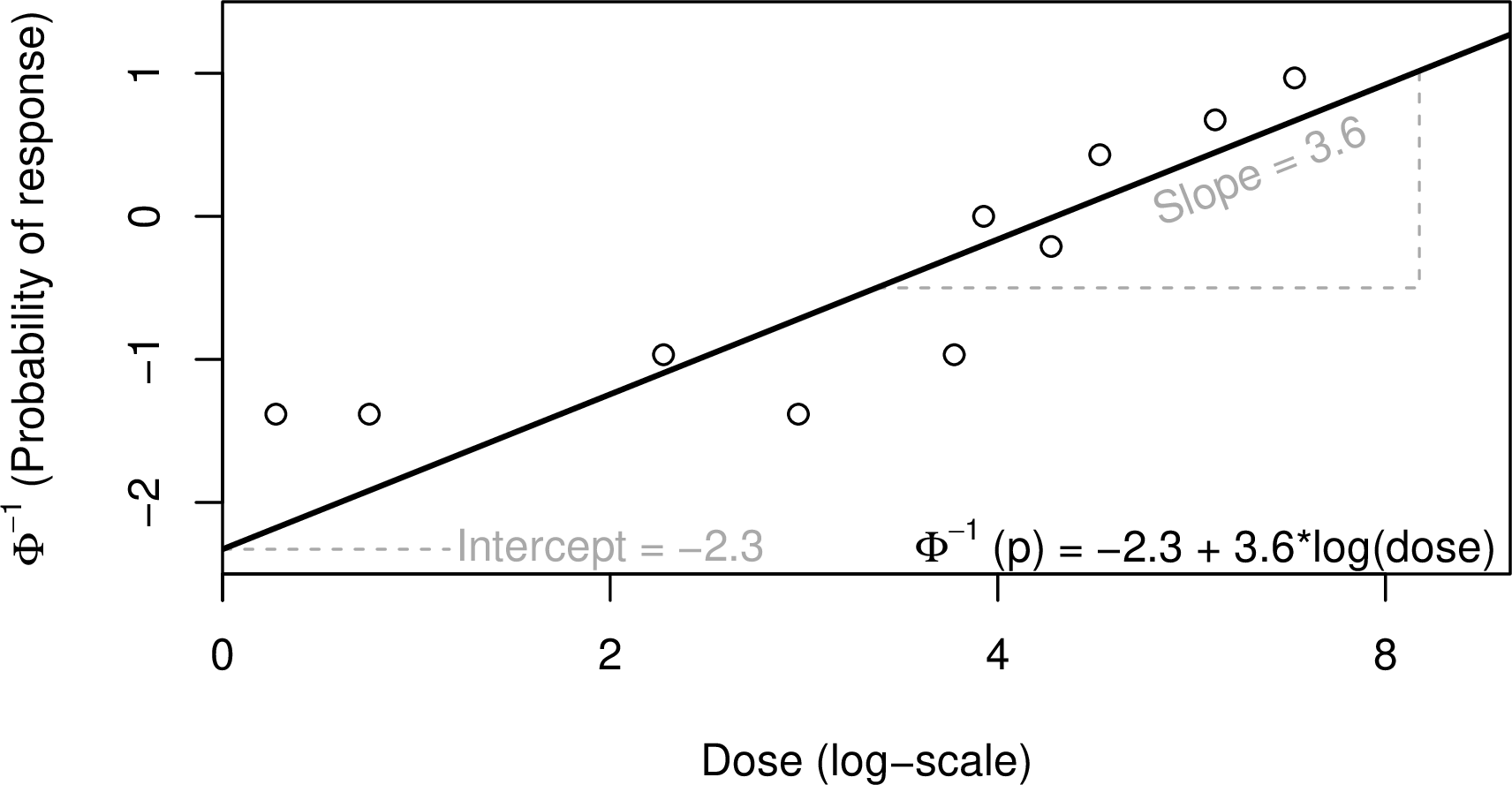
The ‘standard’ probit model has two parameters just like the linear model shown below:

a = intercept

b = slope

but unlike the linear model it has an added cumulative distribution function denoted by the Φ symbol in the equation below for the normal distribution.

A plot of this can be seen in the figure below

The log of the concentration (or concentration) is typically used because this means we are assuming a log-normal tolerance distribution for the test subjects; this assumption is supported by “a long history of experience” [1].

With the standard probit model we assume that the probability of observing a response in the zero concentration (control) group is zero i.e. impossible. This is not necessarily a desirable property in ecotoxicology where we often need to allow for the possibility of a natural response in the control group. Abbott’s correction can be used to adapt the probit model to allow for an observed response greater than zero in the control group. This approach is not recommended, however, because it assumes that the background response is known with certainty whereas in reality it is estimated from the data.

The OECD recommend entering the correction parameter into the model [1]. The correction parameter (also known as the natural response parameter), c in the equation below, is estimated from the data with the a and b parameters. The zero dose is left in the model and used to estimate c, and since we are using a non-linear model, the c estimate affects the a and b estimates, and vice versa.

The concentration-response model with a background response parameter is described as follows:

The figure below shows two lines fitted with probit models to the same data. The grey line represents the concentration-response relationship estimated with a probit model using Abbott’s correction (excluding the Control data at zero dose). The grey points show the underlying data after Abbott’s correction has been applied. The black line represents the model when we also estimate the background response (with the dotted line showing the c estimate, and the points are the raw data values i.e. proportion of response at each concentration).

The EC_X is the concentration associated with a x% response. When we allow for a background response, the definition of the EC_X is slightly more complicated. The EC_X becomes the concentration associated with a x% response in the part of the population that did not respond at concentration zero.

For example, we can calculate point estimates for the EC₅₀ values for both models plotted above. For the model with Abbott’s correction, the EC₅₀ estimate is 4.43 (95% CI: 3.80, 5.16). For the model with the ‘OECD correction’ (i.e. estimated as part of the model), the background-corrected EC₅₀ estimate is 4.62 (95% CI: 3.78, 5.41). The 95% confidence intervals for the EC₅₀ estimates are shown by the coloured sections of each fitted line. Where we estimate the background response as part of the model, the confidence interval is wider; this is because we are allowing for the uncertainty in our estimate of the background rate, as mentioned above Abbott’s correction does not allow for this. In other words, 95% confidence interval for the Abbott’s corrected EC₅₀ is likely to contain the true EC₅₀ value less than 95% of the time.

It is worth noting here that confidence interval estimation for EC_X values can is complicated slightly by the addition of the background parameter, but that’s a subject for another blog post.

References

[1]          Organisation for Economic Co-operation and Development (OECD). 2006. Current Approaches in the Statistical Analysis of Ecotoxicity Data: A Guidance to Application. OECD Series on Testing and Assessment No. 54, Environment Directorate, ENV/JM/MONO(2006)18, Paris, France. 147 pp